|
|
"Retsim" is a set of scripts that construct a biophysically-realistic model of a neuron and its presynaptic circuit. Typically, a light stimulus is transduced by an array of photoreceptors (rods and/or cones or transducers), and the resulting signals are synaptically transmitted to an array of bipolar cells, which in turn transmit their signals to one or more ganglion cells. The arrays of different neuron types are generated as semi-random arrays, given a cell density and a regularity (mean/s.d) or by array size or number. Synaptic contacts are automatically set based on a connection algorithm specified in a paramater table. Experiments are defined by constructing a neural circuit, defining an experimental protocol (e.g. voltage-clamp or current-clamp), and defining stimuli and output plots.
The main script is "retsim.cc" (previously "retsim.n") which defines a set of parameters that control the construction of the stimulus and calls construction subroutines to make the different cell arrays and connect them, defines a procedure to display the model, and defines an experiment to run on it. The "makcel" script constructs the neurons, and the "synfuncs" script makes the connections.
To help you get started setting up and running retsim, an example below spells out all the steps. It shows one example of a neural circuit defined by an experiment file "expt_gc_cbp_flash.cc". Once you see how to run this example, you can look at the other expt*.cc files and compare them.
The ".n" versions of these scripts were originally developed to run with the "nc" interpreter, but have not been maintained. Please use the ".cc" versions.
Script                 Function

retsim.cc              main script, oversees construction, connection, display, and run.
retsim_var.cc          variable definitions, set pointers for command-line values.
makcel.cc              makes arrays of neurons, either realistic or artificial.
synfuncs.cc            connects arrays and individual neurons with synapses based on algorithm.
celseg.cc              makes spheres and cables with biophysical properties.
celfuncs.cc            functions to help make cells.
morphfuncs.cc          helper functions to measure morphology params
maknval.cc             script to create table of parameters "nval.n".
modelfit.cc            Levenberg-Marquardt least-squares fitting usimg simulator as fit function (see "Curve fitting with NeuronC" manual)
namedparams.cc         functions for accessing column and row by name (used for "chanparams" file)
nval_var.cc            parameters for nval, automatically generated by "maknval".
nval_var_set.cc        sets parameters for nval, automatically generated by "maknval".
rectask.cc             functions for recording
stimfuncs.cc           stimulus functions.
plot_funcs.cc          plotting functions.
sb_makfuncs.cc         starburst cell make functions.
sb_recfuncs.cc         starburst cell recording functions.
setexpt.cc             reads, links dynamically loaded experiment files
spike_plot.cc          functions to calculate spike rate
synfuncs.cc            functions to generate synaptic connections

onplot_movie.cc        movie frame functions
onplot_dsgc_movie.cc   DS ganglion cell movie functions (includes "onplot_movie")

expt_gc_cbp_flash.cc   experiment file: defines and sets parameters, sets up and runs experiment.
runconf/nval.n         parameter table, defines cell parameters and synaptic connections
runconf/dens.n         channel density table  (subdir runconf is configurable)
runconf/chanparams     channel param table (voffset, tau)
runconf/morph_filexxx  morphology file

nc library in nc/src:

libnc.a                library of functions required by retsim, generated by compiling nc in nc/src
To run retsim natively under Linux or Mac, you must first compile "nc" "vid", and "retsim":
1. Start a console window (in KDE, "konsole", in Mac, "terminal"). Use this window to run the following commands:
2. Untar the distribution. "tar xvzf nc.tgz<Enter>". If you have downloaded nc.tgz to another folder, place that folder name ahead of nc.tgz, e.g. "tar xvzf "Downloads/nc.tgz"
3. Go to the nc directory (folder), "cd nc<Enter>". Make nc with: "make"; This will compile and link all the files for nc and link them into "nc" and "libnc.a". It will also make plotmod and vid. To make nc on a Mac, see the paragraph below "Compiling and linking nc and retsim". Note that to make nc you must install the C and C++ compilers, along with the X-Windows development package
4. Go to nc/models/retsim. "cd models/retsim (cd ~/nc/models/retsim)"
5. Make retsim with: "make". This will make retsim and all the experiment scripts in the makefile. If you are compiling retsim on a Mac, see "Compiling retsim on Mac OSX" below.
6. Edit your shell startup file to include "~/nc/bin" in your PATH. You can use a programming text editor such as kwrite, kate, gvim, gedit, vim, or joe:
7. If you're using the "bash" shell (the usual default), edit your ~/.profile or ~/.bashrc file(s) to include "~/nc/bin" in the PATH.
8. Or if you're using "csh" or "tcsh", add "~/nc/bin" to your .cshrc file (already set in the virtualbox image). You can find an example file at nc/.cshrc.
9. Then, tell the shell to read the .profile, .bashrc (or .cshrc) file: "source .profile" (or "source .bashrc", or for csh, "source .cshrc"). This is done automatically at every login, so you only have to do it once here.
10. Check to see if your path is set correctly, run "cd ~; nc -h; plotmod -h" should run nc and plotmod. Note that some Linux versions come with a command "nc" in the standard distribution. If you place the ~/nc/bin entry in PATH before the other entries, the "nc" in Neuron-C should run instead.
11. To get proper dynamic linking of your expt*.so files in nc/models/retsim, edit your shell startup file and add "LD_LIBRARY_PATH ." (see Compiling and linking below):
(if using tcsh)  setenv LD_LIBRARY_PATH .            [ add to your ~/.cshrc file ]
(if using bash)  export LD_LIBRARY_PATH="."          [ add in your ~/.profile file ]
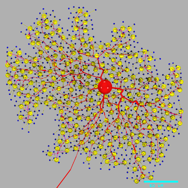
cd ~/nc/models/retsim
retsim --expt gc_cbp_flash --ninfo 2 -d 1 -v | vid
Retsim displays the model on the "vid" window, and prints this text on the screen:
# Retina simulation
#
#   retsim version:    1.7.57
#   nc version:        6.2.18
#   date:              Sat May  9 22:21:20 EDT 2015
#   machine:           dyad
#   experiment:        gc_cbp_flash
#   confdir:           runconf
#   nvalfile:          nval_gc_cbp_flash.n
#   cone  morph:       artif 1
#   dbp1  morph:       artif 1
#   gca   morph:       morph_beta8b,   densities: dens_gca.n
#   chanparams file:   chanparams
#
#
# gcas:
# ganglion cells done.
# xarrsiz = 288; yarrsiz=271; arrcentx=0; arrcenty=0
#
# cones:
# cone spacing: 6.32 um
#
# cones:
# Number of cones: 2074
# photoreceptors done, arrsiz=290.938
#
# dbp1s:
# bipolar cells done.
# Done making neurons.
#
# total cones = 2074
# total dbp1s = 508
# total gcas  = 1
#
# connecting cones to dbp1s
# ........................................................................................
..........................................................................................
........................................................................................
...
...
[i.e. one dot per cone, up to 2074 cones].

# connecting dbp1s to gcas
# ........................................................................................
..........................................................................................
........................................................................................
...
[i.e. one dot per cone bipolar]

# cell type  cone,  2074 cells: div to dbp1 = 1.83
# cell type  dbp1,   508 cells: conv from cone = 7.47, div to gca = 0.524
# cell type   gca,     1 cell: conv from dbp1 = 266
#
#
# Removing neurons that don't connect.
#
# dbp1s  erased 242
# cones erased 890
# total cones = 1184
# total dbp1s = 266
# total gcas  = 1
#
# Done connecting neurons.
#
# cell type  cone,  1184 cells: div to dbp1 = 1.7
# cell type  dbp1,   266 cells: conv from cone = 7.56, div to gca = 1
# cell type   gca,     1 cell: conv from dbp1 = 266
#
Notes:
a. This command line "retsim ... | vid" runs two commands, "retsim" and "vid". The "|" (vertical bar) symbol is a "pipe" that redirects the "standard output" (stdout, defaults to screen) stream from retsim to the "standard input" (stdin, defaults to keyboard) of vid. This is a graphics stream and looks like garbage if printed onto the screen (e.g. try "retsim ... -v" without the "| vid" appended). To stop the display, click on the original terminal window and enter ^C (control-C).
b. The printout of cell and connection information is specified by "--ninfo 2". You can see more details with "--ninfo 3" or "--ninfo 4" in the command line. The display of information on the screen by "--ninfo" is from the "standard error" (stderr) stream of retsim. This separate from "stdout" and is not redirected by the "|" pipe symbol so it is displayed by default on the screen.
c. The printout shows what experiment is being run, and what files were used to construct the model.
d. To get this to run, you must have compiled nc, vid, and retsim, added the ~/nc/bin to your path, and you must have "nval_gc_cbp_flash.n", morph_beta8b, dens_gca.n, and chanparm in the directory nc/models/retsim/runconf. These files are included in the nc.tgz distribution, in nc/models/retsim/runconf, the default directory for these files.
e. The experiment file name is the experiment with "expt_" appended onto the beginning and ".cc" at the end. To run an experiment file, put "--expt" then the experiment name, i.e. "expt_gc_cbp_flash.cc" defines the experiment gc_cbp_flash that you run with "retsim --expt gc_cbp_flash ...". f. Find the other experiment files with "ls -l expt*.cc"
g. The morphology file "morph_beta8b" and the density file "dens_gca.n" are located by default in nc/models/retsim/runconf.
h. To rotate the model, run:
retsim --expt gc_cbp_flash --ninfo 2 --mxrot -90 -d 1 -v | vid
To flip the morphology left-right, run:
retsim --expt gc_cbp_flash --ninfo 2 --flip 1 -d 1 -v | vid
i. To run the experiment and generate plots, run the same command line, except remove the "-d 1":
retsim --expt gc_cbp_flash --ninfo 2 -v | vidj. To capture the output of the experiment in a file, run the same command line, except add ">& file.r":
   retsim --expt gc_cbp_flash --ninfo 2 -d 1 >& file.r  (display model, send the stdout and stderr to a text file)
   plotmod file.r | vid                                 (display the model file as graphics)
   retsim --expt gc_cbp_flash --ninfo 2 >& file.r       (run expt, send plots into a text file)
   plotmod file.r | vid                                 (display the plots in text file as graphics)
To run the experiment in the background do:
   retsim --expt gc_cbp_flash --ninfo 2 >& file.r &              (run expt in background)
same as:
   retsim --expt gc_cbp_flash --ninfo 2 >& file.r; ^Z bg <Enter> (run expt in background)
The ^Z (control-Z) stops the current process, and the "bg" command runs it in the background as if you had run it originally with an "&" (ampersand) after the command. When you run a command in the background, you can run other commands simultaneously.
k. To make a smaller neuron array that runs faster:
   retsim --expt gc_cbp_flash --ninfo 2 --arrsiz 100 -d 1 -v | vid
   retsim --expt gc_cbp_flash --ninfo 2 --arrsiz 100      -v | vid
l. Note that retsim currently lacks interactive display of the model, i.e. you can't redisplay a view with a different rotation or magnification without rerunning the model construction mode. Although on first thought this capability may seem important for developing intuition about the cell model, or to determine where to place a recording electrode, in practice it is not necessary. To set an electrode location, one can specify node numbers in a cell, or one can specify absolute coordinates or by coordinates relative to the cell soma by nearest node position. A set of functions can find recording points specified in this way by absolute or relative location (see "celfuncs.cc").
m. You can find more examples of how to run retsim in "Examples of how to run retsim" below.
scp file.r extmachine:/home/myfolder
or
rsync -azr -e ssh --progress file.r extmachine:/home/myfolder
 (same as: rsyncc file.r extmachine:/home/myfolder)
A command called "rsyncc" runs "rsync" with the appropriate command line switches. This rsyncc command is installed in the virtualbox image:
rsyncc file.r extmachine:/home/myfolder
povray             ray tracer useful for 3D rendering the output of "retsim -R" into .png files
ffmpeg             movie-maker useful for making movies from output of "vid" (see "Making movies" below)
mpeg_encode        movie-maker useful for making movies from output of "vid"
libreoffice        full-featured office lookalike "soffice"
xmgrace            full-featured graphing, fitting, and analysis program.
octave             full-featured matlab almost-lookalike, run from terminal or console window.
vncviewer          virtual console and server, useful for running remote desktop
ninfo = 0   // don't display any information
ninfo = 1   // display basic info on number of cells
ninfo = 2   // display info on cells and connections
ninfo = 3   // display basic debugging info
ninfo = 4   // display debugging info about connections
ninfo = 5   // display debugging info about cell morphology and connections
For example, to see basic cell connection info:
retsim --expt ... --ninfo 2 ... -v | vid
or
retsim --expt ... --ninfo 2 ... >file.r
The information is printed on the computer screen (using the "stderr" stream). For most runs it is helpful to set ninfo = 2, which prints out the convergence and divergence for each cell type. You can set ninfo in the experiment file or in the command line.
retsim -hThis prints out:
## retsim: nc version 6.2.18
nc -v      video mode to stdout (makes graphics).
   --var n  set variable from command line.
   -c      run from inside script with first line = #! nc -c
   -d 1    display 'neural elements' with 'display' statement.
   -d 2            'compartments'
   -d 4            'connections'
   -d 8            'nodes'
   -d 16           'stimulus'
   -d 32           'movie (vcolor,cacolor)'
   -p 1    print out compartments as conductances.
   -p 2    print out compartments as spheres, chan densities.
   -q      quiet, don't print extra info (eqiv to "--info 0").
   -E n -e n override xmax, xmin on plots
   -M n -m n override ymax, ymin on plots
   -l n    set 'lamcrit' variable (0=no condensation).
   -f      no file name on graph.
   -F      no labels on graph.
   -I      run as interpreter only.
   -K      print out all predefined symbols.
   -n      no node numbers on graph.
   -r n    random number seed. Negative = different each time.
   -s n    set precision of output numbers. def=6.
   -C      run input file through CPP preprocessor .
   -R      output symbolic display for "povray" ray-tracer.
   -L n    set line width for display statement.
   -w n    set vid window size for "ncv" or "ndv".
   -W n    tic label char with in terms of screen size.
   -y n    debug level.
   -z n    debug category.
   -1 fn   redirect stdout to file "fn"
   -2 fn   redirect stderr to file "fn"
When running "retsim -h" (or any other linux command) in a small window, you can page its output like this:
retsim -h | more    # page down with spacebar
retsim -h | less    # page down with spacebar or page down key, and go down and up with arrow keys

Exit from "more" with ^C or page to the end.
Exit from "less" with "q".
Note that to display several "-d" features at once, you add the numbers, i.e. to display the neural elements (the cell) and nodes, use "-d 1" and "-d 8", i.e. use "-d 9".
You can also set the font size for the node number by taking a size in the range 0.1 - 5, dividing by 10, and adding this to the node number, then multiply by -1. For example, for a display of the nodes in a cell with a small font, you can set the node display cell_nscale to -3.05. For a display of the cell number in an array of cells, you can use -2.2. For a display of the cell number and node number for each node (2 numbers per node), use -6.05, and for a display of the cell type, cell number, and node number (3 numbers per node), use -7.05. To not display nodes on a cell type, use -9, either for node_scale or cell_nscale.
To set the node number and font size display for a cell type, set the variable "cell_nscale" (cell = cell name, i.e. gca_nscale) with the display template number as described above. You can set this variable on the command line, or in the experiment file in the "setparams()" procedure. To set the node displays for all the cell types, use the variable "node_scale". If set, the "cell_nscale" variable overrides the "node_scale" variable.
  retsim --expt gc_cbp_flash --node_scale -2.1 -d 9 -v | vid
  retsim --expt gc_cbp_flash --node_scale -2.1 --gcb_nscale -3.05 -d 9 -v | vid
retsim ... --disp_zmax -28 --disp_zmin -60To exclude part of a cell, reverse the values, i.e. make disp_zmax smaller than disp_zmin.
retsim ... --disp_zmax -60 --disp_zmin -28Since disp_zmax and disp_zmin function for several cell types, it is useful to have analogous variables for zmax and zmin for each cell type. The dsgc is bistratified so often just one of its dendritic arborizations is displayed. For this specific purpose, use "disp_dsgc_zmax" and "disp_dsgc_zmin":
retsim ... --disp_dsgc_zmax -28 --disp_dsgc_zmin -60
display_z (max, min);
Once you start running simulations, you will also need to view or edit the nval_xxx.n, dens_xxx.n, and possibly the chanparams files in nc/models/retsim/runconf. An excellent editor for opening multiple files is "kate" (however it's not the best one to copy-and-paste). The nval.n file is large and you may need to use a small font to readily see all the columns in the file (cell types).
The retsim script is controlled by a set of variables that tell it which neurons to create and how to connect them. The variables are read from the default neuron parameter table, "nval.n", but are also set by an "experiment file", and from the command line.
An experiment file (e.g. expt_gc_cbp_flash.cc) defines the experiment, with statements to tell retsim which cells to include in the simulation, what stimuli to run, and what plots to generate at runtime, and how to run the experiment -- e.g. a series of voltage clamps. Retsim can then determine (from nval.n) what synaptic connections and biophysical properties (from dens.n) the cells should have. Then the retsim script automatically constructs the neural circuit model, and returns control back to the experiment file, which runs the experiment. The retsim script is designed to be run with many possible different types of experiment. Many experiment files can be created to define different neural circuits or different experiment protocols.
In addition to defining the experiment, the experiment file often defines parameters that allow the user to modify the details of the simulation, i.e. the biophysical details of the neurons, their spacing, or synaptic connections, and the size, frequency, or timing of a stimulus, or the exact form of the output plots. Although it would be possible to make a new experiment file for each variation of parameters, it is usually preferable to create one experiment file and vary it by selecting appropriate values for its parameters.
An experiment file is written in the nc script language (see the Neuron-C manual), and should contain the "defparams()", "setparams()", and "runexpt()" procedures, as explained below. The defparams() procedure defines parameters whose values you will want to change on the command line. The setparams() procedure sets the values of parameters, for example to control how the circuit is constructed, or values to override those in the nval file. The "runexpt()" procedure sets up stimuli and plots, and runs the experiment using a "step" or "run" statement. A good way to start would be to take an existing experiment, e.g. "expt_gc_cbp_flash" or "expt_cbp_vclamp", and modify it to make a different circuit and/or experiment.
Neuron-C has both interpreted and compiled versions. The original interpreter "nc" is excellent for simple models that you may want to set up quickly, for example, a simulation of one neuron or an array of one neuron type (see "nc/models"). For multiple neurons of several types, the compiled version of "retsim" is best. It allows you to quickly set up a neural circuit with biophysical properties and synaptic connections and define an experiment to run.
A compiled experiment file is written as a standard .cc file using a set of C functions. It is then compiled and linked as a dynamically-linked library (in linux, "file.so"). This allows the retsim script to select an experiment file at runtime instead of requiring that retsim be linked separately with each experiment file. A good way to set a new experiment file for compiling is to look in the "makefile" and modify an existing entry for compiling and linking an experment file. If you want to make a new experiment file, a good way is to copy an existing experiment file and add the name of the new one to the makefile, which will then allow "make" to compile it automatically.
The compiled experiment file contains several user-defined procedures. Retsim runs these procedures automatically at runtime:
defparams()   Add the definitions here for experimental parameters that will be set on the command line.
	      This is called before the nval.n parameter file is read,
              so you can set a different nval file name here, or on
	      the command line. Also called before the "setvar()"
              procedure sets variables from the command line.

[Retsim sets the variables from the command line, then reads in the nval.n file]

setparams()   Sets variables controlling construction of the circuit
              after the neuron parameter (nval) file has been read.
	      Called after defparams(), but before the density files
	      are read, and before construction of the neural circuit.

[Retsim reads in the dens.n files, one (or maybe 2) for each cell type]

setdens()     Sets neuron parameters and variables that modify the
	      channel densities after they have been read from the
	      density files. Called after densities have been read in,
              but before construction of the neurons and the circuit.
              Optional.

[Retsim makes the cells and constructs the circuit.]

addcells()    Allows the user to add cells not defined in the nval file. Optional.

[Retsim makes the connections between the cells]

addsyns()     Allows the user to add synapses not defined in the nval file. Optional.

[Retsim removes cells not connected]

addlabels()   Allows the user to define node labels using "label()" for display.
	      See ncfuncs.cc,h. Optional.

[Retsim displays the model if requested (with -d xx)]

runexpt()     Runs the experiment. Make final changes to the model, sets stimuli and plots,
              and defines and runs the experimental protocol.
              Called after circuit is constructed.

[Names of these user-defined procedures are set in "setexpt.cc. These procedures are called
in retsim.cc.]
void defparams(void)
{
  setptr("temp_freq", &temp_freq);
  setptr("ntrials",   &ntrials);
  setptr("dstim",     &dstim);
  setptr("sdia",      &sdia);
  setptr("stimtime",  &stimtime);
  setptr("minten",    &minten);
  setptr("scontrast", &scontrast);
}
void setparams(void)
{
  make_rods = 0;
  make_cones= 1;        /* make cones, cbp, gc */
  make_ha   = 0;
  make_hb   = 0;
  make_cbp  = 1;
  make_gc   = 1;
  DEND      = R_2;      /* set DEND region for density file to be region 2 */
  if (notinit(bg_inten)) bg_inten = 2.0e4;      /* background light intensity */
}
void setdens(void)
{
  if (!notinit(cone_cond)) setval(xcone,SCOND5,cone_cond);		// override synaptic val
  if (!notinit(ca_cond)) celdens[cone][_CA][R_AXON] bg_inten = ca_cond; // override Ca density, S/m2

  // In some cases, it's helpful to have 2 density files for one cell type.
  // This allows one cell to have biophysical parameters such as channels,
  //   and the other cell to have a different combination of densities, for example, none.
  // This is useful when subtracting the voltage-clamp currents to
  //   remove the effect of capacitance.
  // The ndens[][] array sets which density file to use for each cell.

  ndens[dbp1][cn=1] = 0;              // set cn 1 to use dbp1_densfile
  ndens[dbp1][cn=2] = 1;              // set cn 2 to use dbp1_densfile2
}
The addcells() procedure allows the user to add cells that are not defined in the nval file,
before the experiment is run.
void addcells(void)
{
  if (set_amx) make_amx();		// make a new amacrine cell type
}
The addsyns() procedure allows the user to add synapses that are not defined in the nval file,
before the experiment is run.
void addsyns(void)
{
  if (set_amx) make_amx_synapses();	// connect a new amacrine cell type
}
The "runexpt()" procedure can include a "for" statement to run an experiment iteratively (see the Neuron-C manual, and "Running a voltage clamp protocol" below). Typically, a stimulus is generated, and the "step()" procedure is called to run the simulation forward in time. Then inside the loop, the stimulus is run again, possibly with a small variation, e.g. a different clamp voltage for a voltage clamp, and the step procedure is run again. Alternately, all the stimuli can be defined before the experiment runs.
void runexpt(void)
{
    double temp_freq, dtrial;
    double Vmin, Vmax;

  if (notinit(ntrials))     ntrials = 1;       /* stimulus repeats */
  if (notinit(stimtime))   stimtime = .10;       /* stimulus time */
  if (notinit(minten))       minten = bg_inten;  /* background intensity (for make cone)*/
  if (notinit(scontrast)) scontrast = .5;        /* intensity increment */
  if (notinit(temp_freq)) temp_freq = 2;

  dtrial = 1 / temp_freq;
  exptdur = dtrial * ntrials;

  plot_v_nod(ct=xcone,cn=midcone,n=soma,Vmin=-.037,Vmax =-.027,colr=cyan,"", -1, -1); /* plot Vcones*/
  stim_spot(sdia, 0, 0, minten*scontrast, start=t+stimtime,dur=dstim);
  step(dtrial);
}
However, another modeling paradigm tests an existing hypothesis suggested by real recordings. If the model fails or cannot approximate the real data even with revisions, this suggests that the hypothesis, to the extent it is incorporated in the model, is false. To elminate a hypothesis when testing several is helpful in modifying or creating new hypotheses.
In a typical biophysically-based model using retsim, you start with the morphology and basic synaptic connectivity along with a stimulus. From there, you can go several directions, depending on your scientific question. If your question is very specific, for example "What is the dendritic (or axonal) interaction between different currents (e.g. excitation and inhibition, etc)?" you may want to get estimates for the biophysical parameters Ri, Rm, Cm (and maybe a diameter factor). This will allow you to determine the interactions between currents in the peripheral dendrites that are not visible in somatic voltage clamp.
For higher level scientific questions, such as "How does the circuit work, i.e. how does it do what we know it does?", you first need to work on getting it approximately calibrated to give correct responses to the relevant stimuli. You can chose light stimuli, or go with electrodes that maintain voltage or current clamps. If you will want to match real data, you'll have to start by matching the stimuli that evoked the real responses. You'll also need to set up plots of relevant parameters in the model circuit, for example, the voltage at different points within a cell's dendritic arbor, currents from voltage clamps, or neurotransmitter released by a neuron's synapses. Then you modify the circuit, e.g. the synaptic or voltage-gated membrane conductances, and maybe the synaptic placement, and see how this affects the output signals. This will give intuition about how the specific microcircuit properties accomplish its signal processing.
For "What does the circuit do given a specific type of stimulus?" or "What stimulus gives the best signal?" you calibrate the model, then apply different stimuli to see which responses have the maximum SNR. If you want to know which stimulus is best, you can apply the output of the model to an "ideal observer", which compares the responses to 2 stimuli and determines the minimum discriminable change in the stimulus. This defines the SNR of the system. Then change the model and see how this changes which stimulus has the best SNR. You can measure SNR of a real cell(s) or a model with an ideal observer ("discriminator") program (see Smith and Dhingra, 2009).
The output signal of the real cell may not be directly related to the real data you attempt to match, because real data is often taken by an electrode or by imaging calcium. These real data are very helpful, and can be targeted for matching by the model -- but are not necessarily the signal transmitted to the next neuron in the pathway. However, then the model can tell you what the real output of the cell would be (i.e. if you could measure it). Imaging glutamate is closer to the real output of the cell but has other issues, such as, how many cells does the glutamate come from, or what portion of the glutamate does the postsynaptic cell respond to?
In the Stincic et al (2016) paper on the starburst amacrine, the real data were obtained from voltage-clamp at the soma, leading to space-clamp issues in the peripheral dendrites. Given the currents from the voltage clamp, least-squares fitting models were run to determine for each specific cell morphology the best fitting values for Ri, Rm, Cm, dend dia, and Rs (electrode resistance). These models were run without a light stimulus, only using a voltage clamp protocol (5 mV step, fitting the charging current curve). After that, the light responses were fitted, which allowed determining the synaptic conductances. The fits were done with the "lmfit" procedures (nc/src/lm_*.cc), called from the "modelfit.cc" program, run by different perl scripts.
When fitting a model to real data, it helps to have only a few free parameters, for example 4 to 6. Although more parameters can be well-fit using least-squares methods, in a biophysically-based model such as retsim, the parameters are often correlated (e.g. Rm, Cm, and dendrite diameter), so that an increase in one parameter can be compensated for by a decrease in another. This causes the fit to be non-unique, i.e. many combinations of parameters appear to fit the data equally well. To prevent this type of ambiguity, it helps to have constraints on your free parameters, so that their values are limited to a fairly narrow range.
Voltage clamp is widely used to determine dendritic conductances (see Taylor and Vaney, 2002), but when the dendrites or axon are long, the space clamp issue limits the accuracy. The model in the Stincic (2016) paper side-steps that problem because the it contains the biophysical parameters that generate the electrotonic decay that cause the space-clamp problem. Once calibrated (Ri, Rm, Cm, dend dia, Rs, etc), and the model currents measured at the soma are fitted to the real data, the model's synaptic currents and conductances can be readily plotted.
Although nc can implement generic postsynaptic channels, often one wants to use the Markov state-machine channels (AMPA, AMPA5, NMDA, GABA, etc). These have more realistic temporal and noise properties. Start calibrating the model without vesicle or channel noise, then add noise to see how it affects the operation of the circuit, and to check the signal-to-noise ratio (SNR) of the output.
For the most realistic synapse, use Ca channels in the presynaptic compartment. For this to work, the node where the presynaptic part of the synapse is located must contain Ca channels and the SENSCA parameter in the nval*.n file must be set greater than 0 (normally 1; see description of the "nval.n" below). This parameter is multiplied by "dscavg", and the product multiplied by the local calcium concentration next to the cell membrane to set the rate of calcium-driven release.
If you don't need the complexity of a rise in [Ca]i driving release, you can leave out Ca channels and leave SENSCA at its default value of 0. Then the synaptic release will be driven by the presynaptic voltage, using SGAIN and/or SVGAIN.
When Ca sensitivity is not set, the release of vesicles is modeled by either a linear or an exponential function. The exponential function is more realistic, and doesn't have a sharp cutoff at more hyperpolarized voltages. The slope of the exponential function is set in units of mv/e-fold change, normally set between 1 and 4. This is described in the nc manual under "Synapse Statement". In "retsim" the exponential gain is "SGAIN", but when you set "SENSCA" >> 0, the exponential gain is not used, since the [Ca]i is set by calcium channels.
If you know what type of synapses to include in the model, it's usually fairly easy to set them up. If you don't know precisely what type of synapses, you can start out with basic excitatory (AMPA) or inhibitory (GABA) postsynaptic receptors. But then the question is, where are they located? If you know the precise position, you can then start bracketing the conductance of the synapses to give the responses that you want. If you don't know exactly where to put them, try different locations and see how these affect the function and output of the model. You may then want to go back to modify the temporal filters in the synapses to set fast or slow rise and fall times.
To get 2 cells to be connected by more than one synapse, there is a way to set the synaptic spacing on the presynaptic cell, and then the synapse can connect to the postsynaptic cell given the pre-post distance is within a criterion (in the retsim/runconf/nval*.n file).
To adjust the amount of neurotransmitter released, in a generic synapse you can change the gain (in nvalxxx.n, SGAIN) or threshold (STHRESH) for synaptic release. In a synapse driven by calcium from a calcium channel, you can change the calcium channel density, its conductance, or you can shift its voltage activation curve (in chanparams, see below). To scale the synaptic output, you can change the postsynaptic conductance.
For example, in Puthussery et al (2013), modeling a primate bipolar cell, we knew approximately where the Na and Ca channels were, but not the K channels. At first, we placed the K channels near the Na channels in the axon terminal, but found that given the K conductance measured at the soma, the axial resistance of the axon limited the conductance too much -- it was impossible to get the K currents large enough. So we had to move the K channels closer to the soma. That helped the model work much better. Then to get the model to duplicate the Na spikes seen in voltage clamp, it was just a matter of finding the Na conductance density and axonal Ri -- which we did by bracketing. We omitted feedback inhibition from amacrine cells to the bipolar cell axon.
There are some generally accepted densities for membrane channels -- see our paper Van Rossum et al (2003). For ganglion cells the spike generator can be set up in the soma with a medium density of Na channels (80-150 mS/cm2) or in the thin segment of the axon with a very high density (300-1000 mS/cm2). The real cell has Na channels in the soma, but spikes start in the thin segment. The Kdr channel density is usually 10% - 25% of the Na channel density. KA, KCa, and Ca channels are usually present in the spike generator at a much lower density (0.01 - 5 mS/cm2). Other types of neurons such as amarine cells, also generate spikes but may have lower Na and K densities. Some types of bipolar cell also contain sodium channels and can generate spikes, though they are generally electrotonically compact enough not to need spikes for signal transmission.
In a bipolar cell, each synapse must have Ca channels to activate release. This can be simulated using the "SENSCA" parameter in nval*.n. The Ca channel density in the presynaptic terminal is often set at first to ~ 0.5 - 2 mS/cm2. The [Ca]i (internal Ca level) should rest at 20-100 nM, and during synaptic vesicle release should transiently rise to 5-30 uM, with a Ca pump that brings [Ca] down within 50-200 ms.
Although a retsim model can include several sources of noise, it's usually best to start developing a retsim model without including any noise sources, because this simplifies understanding the signal processing it performs. Physiologists often average several recordings of a response to lessen the noise, but in modeling work, it is easy to start without any noise. The most important noise source in a neural circuit is usually synaptic noise, i.e. fluctuation in the timing of quantal vesicle release (in nvalxxx.n, set by SVNOISE). Several other noise sources are provided by the simulator, including fluctuation in vesicle size, thermal Johnson noise, stochastic gating of postsynaptic channels (in nvalxxx.n, set by SCNOISE), and stochastic activation / inactivation of voltage-gated channels. A synapse usually has just a few postsynaptic channels (often not more than 20-50 per synapse), so the binding of neurotransmitter to open (or close) a channel is relatively noisy. However, since one vesicle can gate many channels, vesicle release noise is usually greater than postsynaptic channe noise (see van Rossum et al., 2003).
When you add noise to an existing retsim model, the noise will most likely change the function of the model, in some cases, by a large amount. Synaptic vesicle noise will saturate at the postsynaptic receptor differently than non-noisy transmitter release. Voltage-gated channels are gated differently by a fast-changing noisy membrane potential than a slow-changing membrane potential, because their gating is transient like a high-pass filter. Noise can also help to linearize a circuit with a nonlinear threshold (e.g. nonlinear synaptic release or channel activation), because even when the average signal is below the threshold, noise peaks will rise above threshold and activate the output. Noise in ganglion cells can prevent their spike trains when summed in a cortical cell from generating aliased signals (i.e. beats between close frequencies)
To increase the SNR of a synapse with vesicle release noise, you can increase the release rate, possibly reducing the vesicle size (in nvalxxx.n, SVSIZ). In fact, if you reduce the vesicle size, the synapse will automatically increase the vesicle release rate to keep the amount of neurotransmitter constant. You can also vary the transmitter concentration at the postsynaptic receptor (in nvalxxx.n, STRCONC) to maintain the same average neurotransmitter concentration with different average rates of release. You can vary the randomness of vesicle release with the "vcov" parameter (default=1 in retsim), which sets the release by a gamma distribution instead of a Poisson distribution (see Synapses in nc manual). You can also vary the randomness of release with the "refr" paramter which sets a refractory period between vesicles released at a release site. It is widely assumed, however, that vesicle release is Poisson (random), modulated by voltage through calcium.
Noise is essential in a retsim circuit that you will use to determine SNR and discrimination thresholds. Although photon noise is widely used in "ideal observer" models, and is the largest source of noise at twilight and night, in daylight photon noise is much less, because the photon count is much greater. The noise is proportional to the square root of the mean intensity (or mean release rate). In most cases, photon or other external sensory noise is mixed with biologically generated noise (usually synaptic noise) so the SNR of a signal is the result of a complex mixture of noise sources. Therefore it's essential to set up synapses with realistic release rates, often between 10/s - 100/s in retinal circuits. In brain circuits the release rate may be much lower, activated by presynaptic spikes.
You can plot the vesicle release rate of a synapse by plotting the FA9 parameter (the output of the first temporal filter), and to see the vesicles and their waveshape, you can plot the FB4 parameter (the output of the second temporal filter). You an generate these plots with the "plot_synrate()" procedure (in "plot_funcs.cc").
The number of calcium channels that can drive release at a synapse is usually quite small, in the range of 5-20, so in a synapse that you set up to be driven by calcium, the noise from the small number of channels can have a large effect on the timing of vesicle release.
To avoid the problem of many file names, try to make one version of each file that best fits what you're doing. (You can save old versions by including a date in the file name, but avoid using these old versions except to compare with "diff"). Then try to include in the experiment file variable names for all the parameters you'll need to modify. You can then run the same experiment file with different parameter sets from a script (batch) file using different command lines.
In setting up an experiment in retsim, think carefully about which parameters you will need to change from the command line. Add the parameter definitions at the top of the file, then add the initialization of the symbol table in the "defparams()" procedure. You can see how this is done in the nc/models/retsim/expt*.cc files.
There are 2 ways to set individual parameters read in from an nval file (described in "the nval.n" file below). You can override the nval parameters by overriding their values in memory in the "setparams()" procedure using the "setn()" procedure. The nval file is read in after defparams() but before setparams() (take a look at retsim.cc to understand how this works). A second way is to replace the numeric value in the nval file with a variable name. This variable can then be defined and set in the experiment file -- in defparams(), before the nval file is read in.
You can then arrange to have the values overriding the nval file (with either method above) set on the command line, so that you can readily run the model with different parameter values. This will inevitably require changing the experiment file when you need to add new parameters that you didn't plan on -- so save the old one with a date in the file name, and move on to the new one that has additional parameters that you can change from the command line.
If you end up with an experiment file that's too complicated, i.e. there are too many parameters (e.g. different stimuli, several experimental paradigms, alternate plots, etc.) you may want to split it into 2 or more separate experiment files -- as long as the experiments are identifiably different and easy to remember.
The rule for adding parameters is, feel free to add new parameters as long as they don't change the models and command lines that you have already run. That way, you can always go back and check your work by running the previous command lines, then varying the new parameters to see if everything is working correctly. This is very important, because a model is only as good as your understanding of it, and you will need to check your model to understand whether it is correct.
To add new parameters to an existing experiment, you define the new parameters in the experiment file, initialize them in "defparams()", and set their values to appropriate defaults that keep the model functioning as it did previously before the parameter was added. You can set default values in several ways: you can set the parameter/variable to the default value before the command line is read in, i.e. you set the parameter in "defparms()". Or you can test whether the parameter has been initialized with "notinit()", and if it hasn't you can set its default value, anywhere in "setparams()", "setdens()", or "runexpt()". When a parameter is set ("initialized") either on the command line, elsewhere in the experiment file or in retsim, the "notinit()" function returns 0, but when the parameter hasn't been initialized, "notinit()" returns a 1, allowing an "if" statement to set the default value. This allows you to add a new parameter that is ignored until activated by changing its value.
You can use Neuron-C to run a script similar to a perl script. For example, the neuroman2nc script that converts Neuromantic format to Neuron-C format (see below) is available in perl, awk, and nc versions. By comparing these scripts you can learn how to use these script languages.
1) A cell can be digitized from a photograph or an aligned stack of images. The information is placed into a text file, organized by points, called "nodes", that describe the locations of soma, axon, and dendrites and their branch-points. Each node connects with a cable to its "parent" node, and this information is listed in the file, along with the cable diameter, (x,y,z) location, and the "region", used for supplying biophysical properties:
-----------------------start of morphology file---------------------
#
#  beta cell morphology file,  2006 Oct 4
#
#    node     parent   dia     xbio     ybio    zbio   region      dendr
#
       0        0      21      0        0       -25  SOMA        0
       1        0      2.17    21      -2.47    -8   DEND_PROX   1
       2        1      0.833   22.8     0.0287  -5   DEND_DIST   1
       3        2      1.33    23.3     0.776    0   DEND_DIST   1
       4        0      0.5     13.9    -6.32     0   DEND_DIST   2
       5        0      1.5    -3.25    -33.6   -30   HILLOCK     0
       6        5      0.5    -6.81    -37.6   -30   AXON_THIN   0
       7        6      0.5    -25.5    -66.4   -30   AXON_THIN   0
       8        7      0.5    -121.2   -160.2  -30   AXON_PROX   0
Note that the soma has itself as its parent.
The variables "SOMA", "DEND_PROX", "DEND_DIST", etc. are labels for the regions within the cell. These labels are variables defined in retsim_var.cc. You may change the values of these variables, and you may add your own additional ones in the morphology file. You may also use another set of labels, "R1", "R2", "R3", etc. that are predefined in retsim_var.cc. These regions, defined by either set of labels, are for use in the "dens_xxx.n" file (see below), where each column defines the density of channels and other values such as Rm, Ri, complam, and color for that cell region.
The "dendr" column defines dendrite numbers to be utilized for selectively constructing dendrites. If any of the command-line variables "sbac_dend1,sbac_dend2 ... sbac_dend5" are set, the dendrites with these numbers will be constructed from the morphology file, and other dendrites will not be constructed. If in addition the "sbac_dend_cplam" variable is set, the other dendrites (not set in sbac_dend1-5) that would have not been constructed are now constructed with compartment size set by sbac_dend_cplam. This arrangement is useful for constructing a model with just one or a few dendrites included with small compartments for high resolution, and all the other with large compartments, to minimize the number of total compartments. Other variables gc_dend1-5 and aii_dend1-5 are also defined for use with these cell types.
Depending on the orientation of the stack, you may need to swap the ybio and zbio columns. You can readily do this by editing the neuroman2nc command.
The scale factors for the "neuroman2nc" command are set by default to 1. However, usually the number of microns per pixel differs from 1, so you can set the scale factors from the command line:
neuroman2nc cell_file.swc > morph_cell_file
neuroman2nc --xyscale 0.0495 --zscale 0.05 cell_file.swc > morph_cell_file
scale_morph_file --xscale 12.5 --yscale 12.5             morph_xxx > morph_xxx_scaled
scale_morph_file --xscale 12.5 --yscale 12.5 --zscale 10 morph_xxx > morph_xxx_scaled
scale_morph_file --xyscale 12.5                          morph_xxx > morph_xxx_scaled  # sets x,yscale, leaves zscale
scale_morph_file --xyzscale 12.5                         morph_xxx > morph_xxx_scaled  # sets x,y,zscale
SOMA
DEND
DEND_PROX, DENDP
DEND_MED,  DENDM
DEND_DIST, DENDD
HILLOCK, HCK
AXON
AXON_THIN, AXONT
AXON_PROX, AXONP
AXON_DIST, AXOND
VARICOS, VARIC
Alternately, you can also use these regions:
R1,R2,R3,R4,R5,R6,R7,R8,R9,R10This "R" region set is useful, for example, to label radial regions by distance (see below).
You may also mix the 2 above sets of regions. As variables they are given different integer values. If you prefer, you can define another set of regions as integer variables and use them in the morphology file and the density file.
set_morph_file_reg --radincr 15 morph_xxx > morph_xxx_regionsAnother version, useful for bipolar cells with dendrites that stick out in one direction and an axon that sticks out in the oppositie direction, allows different region sizes for dendrites and axon:
set_morph_file_reg_ax --dendincr 10 --axincr 15 morph_xxx > morph_xxx_regionsYou can also set the scales in this operation:
set_morph_file_reg --dendincr 10 --axincr 15 --xyscale 1.5 --zscale 0.6 morph_xxx > morph_xxx_regions
-----------------------start of morphology file---------------------
#
#    node     parent   dia     xbio     ybio    zbio  region     dendr
#
       0        1      10      0        0        0    PSOMA       0
       1        0      8       0        0        2    SOMA        0
       2        1      2       0        0        4    SOMA        0
       3        2      1.33    23       0.7      0    DEND_DIST   0
       4        0      0.5     13      -6.3      0    DEND_DIST   0
       5        0      7.5     0        0       -3    SOMA        0
       6        5      3       0        0       -6    SOMA        0
       7        6      1.5    20        0       -10   AXON        0
#    node     parent   dia      xbio     ybio    zbio   region      dendr
#
       0        0  SomaDia        0        0      -25   SOMA        0  # soma is variable diameter
       1        0     2.17       21    -2.47       -8   DEND_PROX   1
       2        1    0.833     22.8   0.0287       -5   DEND_DIST   1
       3        2     1.33     23.3    0.776        0   DEND_DIST   1
Then, define SomaDia in the experiment file:
double SomaDia;
...

void defparams(void)
{
   setptr("SomaDia", &SomaDia);
   ...
}

void setparams(void)
{
   if (notinit(SomaDia) SomaDia = 10;		# default value
   ...
}
Then you run retsim like this:
retsim --expt gc_cbp_flash ----gca_file morph_morph_beta8b --SomaDia 11 ...Sometimes it is helpful to set all the dendrite diameters in a morphology file to a variable, for example, "dend_dia". This is useful when you don't have accurate diameter information and want to bracket the diameter values. You must define this variable in the experiment file as explained above.
retsim --expt gc_cbp_flash ----gca_file morph_morph_beta8b --SomaDia 11 --dend_dia 1.5...Note that the "scale_morph_file" and "set_morph_file_reg_ax" commands will preserve any variable names in the "dia" column (col 3) in the morphology file if you don't set "diascale".
dend_dia_factor      // dendrite dia multiplier factor
dendp_dia_factor     // proximal dendrite dia multiplier factor
dendm_dia_factor     // medial dendrite dia multiplier factor
dendd_dia_factor     // distal dendrite dia multiplier factor
ax_dia_factor        // axon dia multiplier factor
cell_dia_factor      // cell dia multiplier factor
These "_dia_factor" multiplier factors are currently set to work with the DENDP, DENDM, DENDD, AXON labels in the morphology file. To use them with the numbered regions R1, R2, ... R10 you can reassign the R1, R2 ... labels in the "setparams()" procedure in the expt_xxx.cc file:
R1 = DENDD;
R2 = DENDM;
R3 = DENDP;
R4 = SOMA;
R5 = AXON;
...
You can also use the ARBSCALE parameter in the nval.n file to scale the dendritic arbor size and the DENDDIA parameter to scale the dendrite thickness.
#    node     parent   dia      xbio     ybio    zbio   region      dendr
#
       0        0       21        0        0      -25   SOMA        0
       1        0     2.17       21    -2.47       -8   DEND_PROX   1
       2        1    0.833     22.8   0.0287       -5   DEND_DIST   1
       3        0      0.5     13.9    -6.32        0   DEND_DIST   2
       3        3      2.5     13.9    -6.32        0   DEND_DIST   2   # make a sphere here
       4        0      1.5    -3.25    -33.6      -30   HILLOCK     0
       5        4      0.5    -25.5    -66.4      -30   AXON_THIN   0
       6        5      0.5    -121.2  -160.2      -30   AXON_PROX   0
You set the cell morphology using the "celltype_file" variable, e.g. for a "gca" cell:
sbac_file = "morph_cell4;or on the command line:
--sbac_file morph_cell4
To set the second cell morphology, you set the "celltype_file" variable, e.g. for the starburst amacrine cell:
sbac_file2 = "morph_sbac_cell5;
morph_frac = 1;
or on the command line:
--sbac_file2 morph_sbac_cell5
--morph_frac 1
You may need to set the following parameters in the nval.n file that are related to the specific morphology. The SOMAZ parameter sets the location of the soma which tells the simulator where to place all the other nodes in relation to the soma -- but the SOMAZ parameter is only for the first morphology. For the second morphology, you set the SOMAZ2 parameter to give the second cell morphology a similar position in the circuit as the first cell morphology. This will allow the second cell morphology to make synaptic connections in the same way as the first morphology. Likewise, you may want to set the ARBSCALE2 parameter to expand or shrink the dendritic arbor size, or set the DENDDIA2 parameter to make the denrites thinner or thicker:
	       /* if == 0, default to 1st morphology */
SOMAZ2         /* soma Z loc */
ARBSCALE2      /* xy scale for dend tree */
DENDDIA2       /* dend dia (thickness) factor */
Retsim first constructs the largest and most downstream neuron set in the experiment file. Typically this is a ganglion cell, but it can also be another neuron such as an amacrine cell (e.g. the starburst amacrine) or a bipolar or horizontal cell. The size of this cell determines how large the model and its arrays of presynaptic cells will be. Next, the presynaptic array is generated, given a cell density and regularity ("REGU", mean/s.d., specified in the nval.n file). Typically the regularity is set to 5-10, but very realistic arrays can be generated with regularities from 3 (almost random), to 50 (triangular array as in foveal cones). The extent of each neural array determines the size of the next higher presynaptic array (typically photoreceptors). The neuron types included in the simulation are defined by the user in the experiment file, by setting the "make_celltype" variables (e.g. make_dbp1 = 1) variables in "setparams()".
If a smaller array is required, a large cell and array of presynaptic neurons can be trimmed using the "arrsiz" parameter, which sets the maximum size in microns for the entire array. Any neurons or parts of a neuron outside this limit are trimmed away before the simulation is run.
After the ganglion cells and amacrine cells have been made, retsim finds the size of the whole array, and then increases the xarrsiz, yarrsiz variables to provide extra space for horizontal cells and bipolar cells that have laterally extending dendrites. One consequence of this is that, for example, adding an additional bipolar type will enlarge the array, which will affect the (semi-random) locations of all the bipolar cell types and photoreceptors. To avoid having the addition of a bipolar cell type affect the placement of other cell types, set the "arrsiz" or "xarrsiz,yarrsiz" variables. This will set array size, preventing it from being increased by the dendrites of horizontal cells and bipolar cells, which will prevent interaction between the different bipolar cell arrays.
Besides the automatic way of generating cell arrays described above, you can set the cell positions in several other ways. You can specify the size of the array for each celltype, making it either square or rectangular, and use the cell density and regularity specified in the nval.n file (using the ___arrsiz, or ___xarrsize and ___yarrsiz arrays, ___=cellname, see retsim_var.cc). The size of the array for the different cell types can vary. Or you can specify cell arrays using exact cell positions, defined by arrays of x-values, y-values, and theta-values (rotations) (using the ___xarr, ___yarr, ___tharr arrays, ___=cellname). This is helpful when you are using an array of several cells of the same real morphology and want to rotate the morphology by different amounts for each cell. You can also set the cell numbers arbitrarily (with ___narr, ___=cellname). This gives you more control over the precise cell and dendrite positions which may be important when generating a synaptically interconnected network of cells. (See expt_aii_dbp.cc).
To view a stereo pair, while looking at the pair of images (one rendered rotated with respect to the other), you can converge your eyes by focusing on your finger about 6" in front of your eyes. While moving your finger closer and farther away while continuing to focus on it, try to fuse the 2 images into one and you can then see them in 3D stereo. If the stereo doesn't look correct, the rotation in rendering may be backwards, so you can try swapping their positions, i.e. making the opposite rotation. Some people can also fuse the 2 images by diverging their eyes. If converging your eyes hurts too much, you can get an inexpensive stereo viewer suitable for viewing prints and computer monitors.
If you instead set the variable "rodarr" to one of the values tested in the setparams() procedure, you can then set rodxarr[], rodyarr[], rodtharr[], and/or rodnarr[], and nrods -- these set the xloc, yloc, angle (not relevant for rods) and cell number, and number of cells, respectively. Of course if you set rodarrsiz, the "rodarr" method doesn't work -- the 2 methods are mutually exclusive.
To make a judgment about how to construct the different cell types in your model, if you need a lot of cells, probably using the "rodarrsiz" is the easiest way. If you only need a few cells, and would prefer them to be located at precise locations (which will not change) then you can use the rodxarr, rodyarr method.
Generally it's easier for photoreceptors to, for example, set rodarrsiz to make a square array of rods. They will then connect to whatever rod bipolars exist within the area of that array. The CELCONV for RBPs is usually set 25, so 25 rods will connect to each RBP. This usually depends on having the RBP morphology grow a new dendrite for each rod -- this is set by GROWPOST=1 for rod input to the RBP. The CELDIV for rods to RBPs is usually set to 2, so only 2 RBPs will connect to each rod.
After the neural arrays are generated and interconnected according to a connection algorithm, the neurons that didn't get connected are removed. This is necessary because the excitatory presynaptic circuit of a ganglion cell only extends typically 20-50 um beyond the ganglion cell's dendritic tips, yet precisely which presynaptic neurons are connected depends on their lateral extent, the specific connection algorithm, as well as the positions of the presynaptic neurons.
During the synaptic connection procedure, for each neuron the numbers of presynaptic and postsynaptic neurons it connects to are totaled and saved in a table. Any neurons that don't connect to a postsynaptic cell are removed. The process is started by first checking the layer immediately presynaptic to the ganglion cell, i.e. the bipolar cells, and afterwards checking the more distal neurons, i.e. the photoreceptors.
To preserve all the neurons, even those that didn't get connected, you can set the parameter "remove_nconns" to 0, either on the command line or in the setparams() procedure.
After the presynaptic arrays of neurons are generated, they are synaptically connected with an algorithm that connects each presynaptic neuron to a nearby postsynaptic neuron(s), and extends the presynaptic axon or the postsynaptic dendritic tree, if appropriate, to create an almost-realistic morphology. Realistic numbers of connections are generated, so that a postsynaptic neuron can receive synaptic connections from several presynaptic neurons, with multiple contacts if appropriate, and a presynaptic neuron can connect to several postsynaptic neurons if appropriate. For example, a bipolar cell receives synaptic contacts from several photoreceptors, but the nearest ones are most likely to make contacts.
One connection algorithm available in retsim calculates a Gaussian probability for making connections, so that each connection is made at random, yet the closest presynaptic neurons are more likely to connect. This allows two random arrays of neurons to be connected with Gaussian weighting functions relatively smoothly. The exact number of connections between a presynaptic and a postsynaptic cell can vary, but the average is closely controlled.
The type of connection algorithm used is specified by the type of presynaptic arbor and the type of postsynaptic arbor. These properties are specified in the nval.n file as DENDARB and AXARBT. A value of 0 means non-branched, 1 means branched, and 2 means highly branched. When connecting a synapse to an unbranched postsynaptic dendritic tree, the postsynaptic tree is extended to generate more branches from the soma if the GROWPOST parameter for that synapse is set. A branched postsynaptic cell will extend new branches from its proximal dendrites. A highly branched postsynaptic cell will not grow branches but will allow synaptic contacts to be made if the presynaptic cell is within a criterion distance (MAXSDIST).
The "synfuncs.cc" file contains the connection procedures. For each pair of cell types, retsim determines whether to attempt to connect them (using a set of predefined variables such as "make_dbp1_gca"), and then looks up the connection parameters in the "nval.n" file. The algorithm for connecting each pair of cell types depends on their dendritic and/or axonal morphology. For example, for presynaptic arbors that are NBRANCHED (not branched) but grow (i.e. for an artificial bipolar cell morphology), retsim will make a new branch from the proximal axon to the synapse onto the postsynaptic cell. If the presynaptic cell (axon) is a relatively unbranched real morphology and the postsynaptic cell has a branched dendritic arbor, the presynaptic cell is connected to the closest point on the postynaptic cell if it is within a criterion distance.
To specify where synaptic connections are made more precisely (without specifying the node numbers), several synaptic connection parameters can limit where connections are made from within the presynaptic cell or to within the postsynaptic cell. These parameters are set in the "nval_xxx.n" file (see below). The SYNREG parameter sets an allowable region for output synapses from the presynaptic cell, and the SYNREGP parameter sets an allowable region to connect to in the postsynaptic cell. For real morphologies, the region is specified in the morphology file in the "region" column, #7, and this can be a number or a variable (R1-R9 or DEND ... AXON, see "retsim_var.h/.cc"). If the region specified by the SYNREG or SYNREGP parameters in the nval_xxx.n file is greater than the number of regions, i.e 100 or more (but less than 1000), then it is taken as a node label in column 8 of the morphology file. Node labels are normally set to the region * 100 + an integer, and are handy to allow specific or representative nodes to be accessed in a similar way between different morphologies. For artificial morphologies, the regions accessed by the SYNREG and SYNREGP parameters are set by the makcell() procedure in makcel.cc.
In addition, synaptic connections can be limited from/to a set of regions, for example, the dendritic arbor, so they are not made from the presynaptic soma or to the postsynaptic axon (except typically for bipolar cells). To specify this behavior, you can set the SREG1-SREG8 rows in the dens_xxx.n file to a non-zero value for any of the cell's regions, which will allow synapses to be made from/to (respectively) that set of regions. The values (range 0 - 1) define the probability that a synapse will be made to or from that region. This allows essentially setting the cell density for making synaptic connections in that region. Then set the entry in SYNREG (for presynaptic) or SYNREGP (for postsynaptic) parameters in the nval_xxx.n file to a number between 1001 and 1008. This will limit synaptic connections from/to the set of regions defined by SREG1 - SREG8 (respectively). Each region The "sreg1 - sreg8" variables are sometimes given the values 1001 - 1008, so the sreg1-sreg8 variables can be entered in the nval.n file.
To check the details of the synaptic connections in a complicated circuit, you can visualize the synapses with a label that contains presynaptic and postsynaptic node numbers. The default icon for a synapse is a line between pre- and postsynaptic nodes with a circle at the midpoint (see "Redefining neural element icons" in the NeuronC Statements and Syntax, and "syn_draw()" in nc/src/ncdisp.cc). You can redefine the synaptic icon to include node labels like this:
void syn_draw2 (synapse *spnt, int color, double vrev, double dscale, double dia,
                                double length, double foreshorten, int hide)

/* draw synapse within small oriented frame */

{
    int fill=1;
    double tlen;
    char tbuf[10];

  if (!draw_synapse) return;
  dia *= dscale;                        /* draw circle with line
*/
  if (dia < 0) dia = -dia;
  color = -1;
  if (color < 0) {
     if (vrev < -0.04) color = RED;
     else              color = CYAN;
  }
  gpen (color);
  if (length > 1e-3) {
     gmove (length/2.0,0.0);
     if (dia > 0.001) gcirc (dia/2.0,fill);
     else             gcirc (0.001,fill);
     gmove (0,0);
     gdraw (length,0);
  }
  else                gcirc (0.001,fill);
  if (spnt->node1a==am) gpen (brown);
  else                  gpen (black);
  sprintf (tbuf,"%d>%d",spnt->node1b,spnt->node2b);     /* print pre and postsynaptic cell number */
  tlen = strlen(tbuf);
  gmove (length/2.0 -tlen*0.3, -1.0);
  gcwidth (2.5*dscale);
  gtext (tbuf);
}


// And in setparams, you activate the new procedure:

void setparams(void) {

{
  ...
  set_synapse_dr (syn_draw2);
}
Then you display the model with: "retsim ... -d 1 -v | vid" and all the synapses
will appear as the icon you've defined in the new "syn_draw2()" procedure.
  for(epnt=elempnt; epnt = foreach (epnt, SYNAPSE, sbac, -1, &pa, &pb); epnt=epnt->next) {
     fprintf (stderr,"syn from %d %d to %d %d\n",epnt->node1b,epnt->node1c,epnt->node2b,epnt->node2c);
  }
Printouts of more complex data from synapses is possible, for example, the relative angles between dendrites connected by synapses (see nc/models/retsim/expt_sbac_stim.cc).
nsynap = synapse_add (dbplist1,dbp1,-1,-1,sbac,1);  /* make list of bipolar synapses onto sbac 1 */

// Then, to make a plot of the total synaptic current and conductance:

 plot_funci(isyn_tot,dbplist1,imax=0,imin=-500e-12); plot_param("Itotbpsyn",green,2,0.3);
 plot_funcg(gsyn_tot,dbplist1,gmax,0);               plot_param("Gtotbp_sb1",blue,1,0.3);
The construction of the neural circuit in "retsim" is done using a table of parameters called "nval.n". Each column contains the parameters for one cell type, and each row gives the values of one parameter for all the cell types. The table can be viewed and modified using a standard text editor, which makes it easy to change/copy values. The "nval.n" table sets the default values for the construction of the neural circuit.
Often it's helpful to create a different nval.n file for each experiment. This allows you to set up different cell densities and synaptic connections. Several nval_xxx.n files are included in the Neuron-C distribution (in nc/models/retsim/runconf).
You can also omit any columns (i.e. any cell type) because the columns are defined (i.e. indexed) by the first row that specifies the cell type. Since the full nval.n file is large and may be difficult to see with a text editor, you can remove columns with the nval_subcol command (in nc/models/retsim/runconf), and you can add new columns with nval_addcol command.
cd ~/nc/models/retsim
make maknval               # this compiles maknval.cc
maknval > nval.n
This makes an nval.n file with default parameters. At the end of the file there are some other files that must be created separately with editing. Follow the instructions at the top of the nval.n file. Copy the nval.n file to nval.h, and edit nval.n to remove everything after the nval parameter rows. Edit nval.h to remove the nval.n parameters, then copy it to nval_var.h, nval_var.cc, and nval_var_set.cc, and edit these files to remove everything but the content below the title of each file and ahove the title of the next.
To compare nval.n files, use the command "diff":
diff nval.n nval_new.n | less
The first block of the nval.n parameters describes how a neuron is to be constructed, some of its biophysical parameters, and also the density and maximum number of cells in an array. The second block, starting with CELPRE1, sets the input synaptic connections for a neuron. The third, fourth, and all the other blocks of parameters starting with CELPOST(1,2,3...) define the output synaptic connections. Note that the default values are set by the "maknval.cc" (maknval.n) file that generates the nval.n file.
First block of parameters in nval.n, for constructing cells:
_MAKE      # whether to make this cell type
_MAKE_DEND # whether to make dendrites
_MAKE_AXON # whether to make axon
_MAKE_DIST # whether to make axon distal
_NMADE     # number of cells made
_MAXNUM    # maximum number of cells of this type
_NCOLOR    # color of this cell type for display, can be parameter, see "Setting cell color" below
_MAXCOV    # max coverage factor (for arrays)
_MAXSYNI   # max number of syn input cells per celltype
_MAXSYNO   # max number of syn output cells per celltyp
_DENS      # density of this type (per mm2)
_REGU      # regularity (mean/stdev) of spacing
_MORPH     # morphology (=0 -> file, or >0 -> artificial)
_COMPLAM   # compartment size (default=complam)
_BIOPHYS   # add biophys properties (use channel density file dens_xxx.n)
_CHNOISE   # add membrane channel noise properties
_RATIOK    # set K density values as ratio from Na
_VSTART    # initial resting potential, when BIOPHYS==0
_VREV      # membrane potential for Rm (VCl), when BIOPHYS==0
_NRM       # the cell's Rm when BIOPHYS==0
_SOMADIA   # Soma diameter for artificial morphology
_SOMAZ     # Z location (x,y loc determined by array)
_SOMAZ2    # Z location of second morphology (x,y loc determined by array)
_DENDARB   # type of dendritic tree, non-branched, branched, etc (retsim.h).
_DENDARBZ  # dendritic arborization level for artificial morphology (synfuncs.cc)
_DENZDIST  # maximum input synaptic z dist for postsynaptic cell. (synfuncs.cc)
_STRATDIA  # stratif. annulus dia (fract of treedia) for artificial morphology. (synfuncs.cc)
_DTIPDIA   # diameter of dendritic tips for artificial morphology (makcel.cc,synfuncs.cc)
_DTIPLEN   # length of dendritic tips for artificial morphology (makcel.cc,synfuncs.cc)
_DTREEDIA  # diameter of dendritic tree (for artificial and real morphology, allows synaptic connection).
_ARBSCALE  # scale factor for expanding or shrinking size of dendritic arbor of real morphology
_ARBSCALE2 # scale factor for expanding or shrinking size of dendritic arbor of second morphology
_DENDDIA   # scale factor for making dendrites thicker or thinner for real morphology
_DENDDIA2  # scale factor for making dendrites thicker or thinner for second morphology
_AXARBT    # type of axonal tree
_AXARBZ    # axonal arborization level for artificial morphology
_AXTIPDIA  # diameter of axonal tips for artificial morphology
_AXARBDIA  # diameter of axonal arbor (for synaptic connections. (synfuncs.cc)
_MAXSDIST  # maximum output synaptic (x,y) distance for presynaptic cell. (synfuncs.cc)
_TAPERSPC  # space constant of diameter taper for artificial morphology.
_TAPERABS  # abs diameter for taper for artificial morphology.
_NDENDR    # number of first-order dendrites for artificial morphology.
_GROWTHR   # distance thresh for growth of dendrites for artificial morphology.
_SEGLEN    # length of dendrite segments
Second block of parameters in nval.n, describing synaptic inputs to a cell type. Each of these ends in a number which is the "synaptic input number" for a cell type. There are 10 possible inputs.
_CELPRE1   # cell type to connect to (negative -> no connection)
_CONPRE1   # connection number of presyn cell
_CELCONV1  # number of presyn cells to connect to
_GROWPOST1 # grow when making conn from presyn cell
Blocks for synaptic output parameters, note that each block ends with the same number which is the "synaptic output number". There are a maximum of 9 possible outputs, each consisting of these parameters:
_CELPOST1  # cell type to connect to (negative, no connection)
_CONPOST1  # connection number for postsyn cell (its synaptic input number from above)
_CELDIV1   # number of postsyn cells to connect to (maximum)
_GROWPRE1  # grow when making conn to postsyn cell
_SYNREG1   # region for synapse in presy cell (if > 0, allows synapses only from this region/label, < 0 any)
_SYNREGP1  # region for synapse in postsyn cell (if > 0, allows synapses only to this region/label, < 0 any)
_SYNSPAC1  # synaptic spacing in presyn dendritic tree (if positive, this enables many synaptic outputs per cell)
_SYNANNI1  # inner rad of annulus in dendritic tree (allows synapses outside this radius)
_SYNANNO1  # outer rad of annulus in dendritic tree (allows synapses inside this radius)
_SYNANPI1  # inner rad of annulus in postsynaptic dendritic tree (allows synapses outside this radius)
_SYNANPO1  # outer rad of annulus in postsynaptic dendritic tree (allows synapses inside this radius)
_SYNANG1   # angle for presynaptic dendrite relative to its soma (sets allowable angle in degrees)
_SYNRNG1   # range of allowable angles (if positive, sets allowable range, if neg, sets range rel to post dendr)
_USEDYAD1  # synapse is dyad using preexisting type
_DYADTYP1  # type of dyad synapse to connect with (sets which type of presynaptic cell for dyad 1->2 cells )
_AUTAPSE1  # synapse back to presynaptic node (allows cell to connect to itself)
_SYNNUM1   # number of synapses per connection (sets more than 1 synapse per connection, typical for bipolar cells)
_SENSCA1   # synaptic release calcium sensitivity (use [Ca]i for driving release instead of expon function)
_SRRPOOL1  # synaptic readily releasable pool (sets initial size of pool)
_SRRPOOLG1 # synaptic readily releasable pool gain mult (default 0 -> rrpool sets gain; 1-> constant gain)
_SMRRPOOL1 # synaptic readily releasable pool maximum (sets max size of pool)
_SMAXRATE1 # maximum synaptic release rate (sets replenishment rate, 0 -> no rrpool)
_SGAIN1    # synaptic gain (sets exponential gain, mV/efold increase, when not using [Ca] sensitivity)
_SVGAIN1   # synaptic vgain (sets additional linear gain factor, if set<=0, set linear synapse using SGAIN)
_SDURH1    # synaptic high pass time const. (sets high pass filter for release)
_SNFILTH1  # synaptic high pass nfilt (sets number of high-pass filters for release)
_SHGAIN1   # synaptic high pass gain (sets high pass filter gain relative to unfiltered release)
_SHOFFS1   # synaptic high pass offset (sets offset in mV for high pass func for release)
_SVSIZ1    # synaptic vesicle size (sets vesicle size without changing overall release, i.e. changes release rate)
_SCOND1    # synaptic conductance (maximum conductance when potsynaptic receptor is saturated)
_SCMUL1    # synaptic conductance multiplier for region of cell
_SCGRAD1   # synaptic conductance gradient from soma
_STHRESH1  # synaptic threshold (threshold for exponential release in mV).
_SVNOISE1  # 1->allow vesicle noise, override, vnoise=0
_SCOV1     # 1=Poisson, <1->more regular, gamma dist (sets properties of noise distribution for release)
_SDUR1     # synaptic event time const. (sets lowpass filter of vesicle release: shape of mini-PSP)
_SFALL1    # synaptic event fall time const. (sets separate first order fall time for mini PSPs)
_SNFILT1   # synaptic vesicle nfilt (sets number of lowpass filters for mini waveshape)
_STRCONC1  # synaptic transmitter concentration. (multiplier for neurotrans conc with ligand-gated channel)
_SRESP1    # synaptic response (ampa,gaba,gj,etc). (sets which Markov state diagram to use)
_SPCA1     # synaptic postsyn Ca relative permeability (default dpcaampa, dpcanmda, etc. range 0 - 1)
_SCAVMAX1  # synaptic postsyn Ca pump Vmax  (default dcavmax, 2e-7, rate per comp area)
_SCAKM1    # synaptic postsyn Ca pump Km (default dcapkm, 1e-6)
_SCNFILT1  # second mesng. nfilt (number of lowp filters in postsynaptic cascade)
_SCDUR1    # second mesng. time const.(time const of filter in postsynaptic cascade)
_SCGAIN1   # synaptic second messenger gain (gain of second messenger)
_SCOFF1    # synaptic second messenger offset (offset of second messenger)
_SCNOISE1  # 1->allow channel noise, override, cnoise=0 (sets noise of postsynaptic channel)
_SNCHAN1   # number of channels (sets number of postsyn channels)
_SUNIT1    # synaptic channel unitary conductace (sets conductance of unitary channel)
_SVREV1    # synaptic reversal potential (usually either 0 for excitatoryh, or -0.065 for inhibitory)
For each input synapse type, you must set _CELPRE and _CONPRE. The _CONPRE parameter refers to the number of the _CONPOST parameter of the presynaptic cell (i.e. _CONPOST2 = the second output synapse).
For each output synapse type, you must set _CELPOST and _CONPOST. The _CONPOST parameter refers to the number of the corresponding _CONPRE parameter for the postsynaptic cell (i.e. _CONPRE1 = the first input synapse).
Although at first thought there seems to be no need to have synapses described with both their presynaptic and postsynaptic connection numbers, the advantage of this format is that the nval.n file lists all the inputs and all the outputs separately for each cell type. Thus, once you have correctly specifed both input connection number and output connection number, you can see a convenient listing of all inputs and outputs for a cell type.
------------------------------------------------------------------
For the input from dbp1 -> dsgc (under the dsgc column):
#
#  dsgc
#
   dbp1     _CELPRE1   # cell type to connect to (neg, no conn)
      2     _CONPRE1   # connection number of presyn cell

------------------------------------------------------------------
For the output from dbp1 -> dsgc (under the dbp1 column):
#
#   dbp1
#
    dsgc   _CELPOST2  # cell type to connect to (neg, no conn)
       1   _CONPOST2  # connection number for postsyn cell
------------------------------------------------------------------
Note: The synaptic biophysical parameters are specified only for the synaptic
outputs. However, some connection parameters are specified for the synaptic
inputs (CELCONV = number of presyn cells to connect; GROWPOST = whether to grow
the postsynaptic cell to make the connection.You can set all the parameters for nval.n in the "maknval.cc" file, so that when you run "maknval > nval.n" you get correctly set parameters. However, it is often easier to start with an existing "nval.n" file and manually edit to add parameter values and new connections. The "nval.n" file is a 2D matrix so it is easy to see the parameter values in neighboring columns and rows.
For branched presynaptic and postsynaptic cells, the SYNSPAC parameter allows you to set multiple synaptic outputs per cell, at a spacing in microns specified by SYNSPACx. Creation of synapses will be subject to the distance limits MAXSDIST (for presynaptic cell), and DENZDIST (for postsynaptic cell), as well as the SYNREG, SYNANN, and SYNANG parameters (described below).
_SYNSPAC1 # synaptic spacing in presyn dendritic tree (if positive, this enables many synaptic outputs per cell)The SYNREG parameters allow you to specify a presynaptic (SYNREGx) or postsynaptic region (SYNREGPx) for the synapse. If either of these parameters is greater than zero, the synapse is created only when the parameter value is equal to the cell's region, defined in the morphology file.
When the SYNREG/SYNREGP parameter value is greater than the number of regions, it is taken to specify the node label, found in the eighth column of the morphology file. The label gets identified, and the corresponding node number is determined. The synapse is created if the node number corresponding to the eighth column label in the morphology file is equal to the synaptic node. If SYNREG or SYNREGP are in the range 1001 to 1008, they limit synaptic connections to a set of regions defined non-zero in the dens_xxx.n file for the SREG1 to SREG8 row parameters (respectively). This is useful to limit synapses from/to the dendritic arbor or to allow them to be made to the soma.
_SYNREG1   # region for synapse in presynaptic cell (if positive, this allows synapses only from this region/label)
_SYNREGP1  # region for synapse in postsynaptic cell (if positive, this allows synapses only to this region/label)
The SYNANN parameters when set greater than zero define a permissible annulus for synaptic locations, specified as a radius from the soma:
_SYNANNI1  # inner rad of annulus in dendritic tree (allows synapses outside this radius)
_SYNANNO1  # outer rad of annulus in dendritic tree (allows synapses inside this radius)
_SYNANPI1  # inner rad of annulus in postsynaptic dendritic tree (allows synapses outside this radius)
_SYNANPO1  # outer rad of annulus in postsynaptic dendritic tree (allows synapses inside this radius)
If SYNANNO > 0 and SYNANNO < SYNANNI, then they define an "exclusion annulus" where synapses are not permitted.
The SYNRNG parameter when greater than zero defines the allowable range for SYNANG (in degrees) for the presynaptic dendrite, measured from the synapse relative to its soma.
SYNRNG cases:

    0 ≥ SYNRNG > -1000  Ignore SYNANG but set the allowable range (-SYNRNG) for
                        contacting a postsynaptic dendrite (synapse relative to
                        its soma) of the same orientation as the presynaptic dendrite.

-1000 ≥ SYNRNG > -2000  Ignore SYNANG but set the allowable range (-SYNRNG-1000) for
                        contacting a postsynaptic dendrite of the opposite orientation.

-2000 ≥ SYNRNG > -3000  Ignore SYNANG but set the allowable rnage (-SYNRNG-2000) for
                        indirectly contacting a cell of the same orientation as the
                        pesynaptic dendrite. The contact is made through a third cell
                        that receives a synapse from the first cell and contacts the second cell:
_SYNANG1   # angle for presynaptic dendrite relative to its soma (sets allowable angle in degrees)
_SYNRNG1   # range of allowable angles (if positive, sets allowable range, if neg, sets range rel to post dendr)
There are several ways to override individual parameter values in "nval.n" for a specific simulation. You can override the nval.n values in the memory array with calls to the "getn(ct, PARM)" and "setn(ct, PARM, val)" functions in the "setparams()" procedure. This procedure runs after the nval.n file has been read into memory. A useful way to do this is to define new variables and use them to set the corresponding value in the nval.n file. You define the variables at the top of the experiment file:
   int sbac_color;
   double soma_z;
Then you add the variable names to the symbol table to allow setting the variables from the command line. This sets the variables to an "uninitialized" value:
   void defparams(void)
   {
     ...
     setptr("sbac_color",  &sbac_color);
     setptr("soma_z", &soma_z);
     ...
   }
Then, you test to see whether the parameters have been set from the command line. The
"notinit()" function returns a "1" (true value) if the variable has not been
initialized, so "!notinit()" returns a 1 (true) if the variable has been set on the
command line:
   void setparams(void)
   {
     ...
     if (!notinit(sbac_color)) setn(ct,NCOLOR,sbac_color);   /* set cell display color */
     if (!notinit(soma_z))     setn(ct,SOMAZ,soma_z);        /* set cell soma z location */
     ...
   }
Then you can set these variables from the command line:
retsim --expt ... --sbac_color 4 --soma_z -45.5 ...
#    rbp    dbp1    dbp2    hbp1    hbp2     a17     aii     sbac    am     amh     ams     gca     gcb    dsgc  gcaoff  gcboff
#
     0       0       0       0       0       0       synrng  synrng  synrng 0       0       0       0       0       0       0   _SYNRNG3   # range of angles for postsynaptic cell
This is especially useful when setting multiple parameters in the nval.n variable all
at once to the same value. You define and set default values for the variables
in "defparams()" which is run before nval.n is read into memory. However, by default
the command line values are set after defparams(), so to allow them to be set
from the command line before testing their values (i.e. setting default values)
in defparams(), you must call "setvar()" in defparams():
   void defparams(void)
   {
   setptr("sbac_synrng", &sbac_synrng);
   ...
   setvar();					// sets values from command line
   if (notinit(sbac_synrng)) sbac_synrng = 30;
   }
If you don't need to test the values or set default values of variables you've
placed in the nval.n file, i.e. you'll always be setting the correct value from
the command line, you don't need to call setvar() from defarams().
The variables you set up and/or access in defparams() can then be set on the command line:
retsim --expt ... --sbac_synrng 15 ...
maknval > nval.n
cp nval.n nval.h
Then remove the numerical parameter definitions from the end of nval.n using a programming text editor such as vi or kwrite. Next, remove the nval.n table at the beginning of nval.h. Next, copy nval.h to "nval_var.h", "nval_var.cc", and "nval_var_set.cc" and edit these files to leave only their correct contents, shown in comments in the beginning of nval.n. Then remove this content from nval.h. Last, "make clean" and "make retsim". This description is included in the beginning of "nval.n".
The last (right) column in the nval.n file is the name of the parameter. This name is a variable that has an integer value, which is preset by default. To add a new parameter, you can edit the nval.n file and add a new row. Then you edit the maknval.cc file to add the new parameter, and run "maknval > nval.n". Then copy the nval.n file to nval.h, and edit nval.h to give new versions of nval.h, nval_var.h, nval_var.cc, and nval_var_set.cc.
You can simplify the nval.n file to remove the columns and rows that are not required for your experiment. This does not require any changes to nval.h, nval_var.h, nval_var.cc, or nval_var_set.cc. The rows and columns can be in any order (except for the first row and the last column, which contain the labels). This works because the rows and colums are described by labels, and when retsim reads in the nval.n file, the data from the file is placed in the correct row and column by referring to the labels. The labels are predefined as variables with integer values in nval_var_set.cc. You can also leave out any rows not needed for the simulation that have zero default values, because the rows for any missing labels are automatically left zero when the file is read into an array in working RAM memory.
For example, to duplicate column 5:
nval_addcol 5 nval.nYou can remove a column from an existing nval file with "nval_subcol".
For example, to remove column 5:
nval_subcol 5 nval.n
Cones are generated by the "makcell()" procedure in nc/models/retsim/makcel.cc. There are several types, defined by their morphology number (MORPH" in the nval_xxx.n file).
To generate an array of cones with randomly specified type, set the cone density (DENS) and nearest-neighbor regularity (REGU) for the standard type "xcone" in the nval_xxx.n file. Then, set the fraction of each sub-type (cone_L,cone_M,cone_S: i.e. red,green,blue) with the "frac_cone_L, frac_cone_M, frac_cone_S" parameters in the "setparams()" procedure in the "expt_xxx.cc" file:
For example:
void setparams(void) {

  make_cones = 1;

  [...]

  frac_cone_L = 0.47;
  frac_cone_M = 0.47;
  frac_cone_S = 0.06;
}
The fractions for the 3 cone types must add up to 1.0; otherwise some of the cones will have the standard "xcone" pigment. The default value for these cone type fractions is zero, which causes each cone to have the default cone pigment type. This standard "xcone" default pigment type can be set with the "cone_pigm" parameter (default value 1):
When the cone array is generated, each cone is randomly assigned to one of the cone subtypes with pigment type according to its fraction. To change the type of pigment used in each cone subtype, you can set the "cone_L_pigm, cone_M_pigm, cone_S_pigm" parameters in the "setparams()" procedure:
Default pigment values:
cone_L_pigm = 1;         // 1,2,3 => monkey; 4,5,6 => turtle; 11,12 => rabbit; 14,15 => guinea pig
cone_M_pigm = 2;         //   16,17,18 => goldfish; 19,20,21 => van Hateren with adaptation
cone_S_pigm = 3;         //   24 human S cone
For more information about the cone pigment types, see "Pigment sensitivity functions" under "Phototreceptor Statement" in the NeuronC manual.
Note that once a cone and its pigment are assigned to one of the "cone_L, cone_M, cone_S" sub-types, its morphology, biophysics, and connectivity are set by the corresponding column in the "nval_xxx.n" file, and by the corresponding "dens_xxx.n" file.
To set the macular and lens spectral filters for cones, you can use morphology (MORPH) 4, and then set the "cone_filt" variable in the setparams() procedure (default: 0 no filter). For more information, see nc/src/wave.cc.
filt    condition
0       no filter (default)
1       macular pigment (see wave
2       lens (small pupil)
3       macular pigment + lens
4       lens (open pupil)
5       macular pigment + lens (open pupil)
To make a file containing a list of the synapses, define the "syn_savefile" variable, either in the experiment file or on the command line. Then, to create the synapses from the list, define the "syn_restorefile" variable.
To save the synapses, create the save file by defining its name:
retsim --expt xxx ... --syn_savefile save_expt_xxx ...To restore the synapses from the file, define the restore file:
retsim --expt xxx ... --syn_restorefile save_expt_xxx ...
Note that when the "biophys" parameter in the nval.n file is set to 0, then retsim does not read the dens_xxx.n file, and takes the "vstart", "vrev", "Rm", and "Cm" parameters from nval.n instead of a density file.
The "density file" (retsim/runconf/dens_xxx.n) defines the biophysical (and some other) properties of a cell, region by region. Each column defines the biophysical properties of one region. The first (left) column of the density file is the name of the biophysical parameter, such as NA, KDR, or RM. These labels are the names of variables that have been set by default to have a value to index into the internal list of channel types. Some of the names, for instance, NA, KDR, KA, SKCA1, are aliases for other internal variables that contain the correct index number. The alternative internal values are in the last column, the comments to the right of the "#". The other columns (2-11) of the density file define conductance density values for each membrane channel type to be inserted into the cables and spheres of the model in the appropriate region.
The rows and columns of the density file can be in any order, and unused rows or columns can be deleted, because each column and row is indexed by the label at the top or left column, respectively. Any rows or columns undefined in the density file are set to zero.
For a listing of all the possible rows (channels and cell properties by region), see the "dens_default_full.n" file in nc/models/retsim/runconf. For a listing of all the channel types, see "Channel statement" in the Neuron-C manual.
Retsim uses dynamic calcium pumps and buffering. Internal calcium-induced calcium-release (CICR) can also be set. In real cells, the calcium pump is electrogenic, that is, the positive calcium ion flux it pumps out of the cell is added to the total cell current. Since calcium is divalent and positively charged, the calcium pump hyperpolarizes the cell. To prevent this electrogenic function, the parameter "dicafrac" is set by default to 0. To enable the electrogenic effect of the pump, set dicafrac = 1. To see more details about the calcium pump and buffering parameters, see "Calcium pumps" under "Channel statement" in the Neuron-C manual.A typical dens.n file for retsim is:
# Default membrane properties (density) file
#
# Densities of currents for the cell's different regions (S/cm2).
#
#      DEND_DIST DEND_PROX SOMA HILLOCK AXON_THIN AXON  AXON_DIST VARICOS R9  R10  (LGRAD,EGRAD)
#
0       R1      R2      R3      R4      R5      R6      R7      R8     R9     R10
#
_NA     0e-3    0e-3    0e-3    0e-3    0e-3    0e-3    50e-3   0e-3   0e-3   0e-3  # Na2
_NA5    0e-3    0e-3    0e-3    0e-3    0e-3    0e-3    0e-3    0e-3   0e-3   0e-3  # Na5
_NA6    35e-3   0e-3    0e-3    4e-3    4e-3    0e-3    0e-3    0e-3   0e-3   0e-3  # Na6
_NA8    0e-3    0e-3    0e-3    0e-3    0e-3    0e-3    0e-3    0e-3   0e-3   0e-3  # Na8
_KDR    15e-3   0e-3    0e-3    15e-3   15e-3   20e-3   10e-3   0e-3   0e-3   0e-3  # K1
_KA     35e-3   0e-3    0e-3    35e-3   35e-3   0e-3    0e-3    0e-3   0e-3   0e-3  # K3
_KH     0e-3    0e-3    0e-3    0.09e-3 0e-3    0.8e-3  0e-3    0e-3   0e-3   0e-3  # K4
_SKCA1  0.12e-3 0e-3    0e-3    0.12e-3 0.00e-3 0e-3    0e-3    0e-3   0e-3   0e-3  # KCA4
_SKCA2  0.01e-3 0e-3    0e-3    0.04e-3 0.02e-3 0e-3    0e-3    0e-3   0e-3   0e-3  # KCA5
_BKCA   0e-3    0e-6    0e-3    0e-3    0e-6    0e-6    0e-6    0e-6   0e-3   0e-3  # KCA3
_CA_L   0.014e-3 0e-3   0e-3 0.014e-3 0.014e-3  0e-3    0e-3    0e-3   0e-3   0e-3  # Ca1
_CA_T   0e-3    0e-3    0e-3    0e-3    0e-3    0e-3    0e-3    0e-3   0e-3   0e-3  # Ca5
_CAP    2e-7    0e-3    0e-3    1e-7    1e-7    0e-12   0e-3    0e-3   0e-3   0e-3  # Capump, sets flux rate
_CAPK   1e-6    0e-3    0e-7    1e-6    1e-6    0e-3    0e-3    0e-3   0e-3   0e-3  # Capump km, sets pump affinity
_CABV   0e8     0e-3    0e8     1e8     1e8     0e-3    0e-3    0e-3   0e-3   0e-3  # Cabuf vmax, sets buffer velocity
_CABK   0e-2    0e-3    0e-7    3e-6    3e-6    0e-3    0e-3    0e-3   0e-3   0e-3  # Cabuf kd, sets buffer affinity
_CABT   0e-2    0e-3    0e-7    10e-6   10e-6   0e-3    0e-3    0e-3   0e-3   0e-3  # Cabuf btot, tot buffer in shells
_CABI   0e-2    0e-3    0e-7    5e-6    5e-6    0e-3    0e-3    0e-3   0e-3   0e-3  # Cabuf btoti, tot buffer 1st shell
_CASH   0       0       0       0       0       0       0       0      0      0     # Ca shells, >0 => sets number of shells
_CAE    0e-7    0e-3    0e-3    0e-7    0e-7    0e-12   0e-3    0e-3   0e-3   0e-3  # Caexch
_CADIA  0       0       0       0       0       0       0       0      0      0     # Cadia, mult for cacomp dia
_CAS    0e-2    0e-3    0e-7    0e-3    0e-3    0e-3    0e-3    0e-3   0e-3   0e-3  # CICR init [Ca]
_VM2    0e-2    0e-3    0e-7    0e-3    0e-3    0e-3    0e-3    0e-3   0e-3   0e-3  # CICR Vmax uptake
_VM3    0e-2    0e-3    0e-7    0e-3    0e-3    0e-3    0e-3    0e-3   0e-3   0e-3  # CICR Vmax release
_VST    dvs     dvs     dvs     dvs     dvs     dvs     dvs     dvs    dvs    dvs   # Vstart, starting voltage
_VRV    vk      vk      vk      vk      vk      vk      vk      vk     vk     vk    # Vrev, battery voltage for Rm
_RM     drm     drm     drm     drm     drm     drm     drm     drm    drm    drm   # Rm
_CM     dcm     dcm     dcm     dcm     dcm     dcm     dcm     dcm    dcm    dcm   # Cm
_DIA    ddia    ddia    1       axdia    axdia  axdia   axdia   ddia   ddia   ddia  # Dia, multiplier
_CPL    cplam   cplam   cplam   cplam   cplam   cplam   cplam   cplam  cplam  cplam # cplam, compartment lambda
_CMUL   1       1       1       1       1       1       1       1      1      1     # syncond, synaptic cond multiplier
_COL    green   blue    red     blue    blue    magenta yellow  gray   ltred  brown # color
_SREG1  1       1       0       0       0       0       0       0      0      0     # regions that allow synaptic input
The density file includes some other rows that define properties for the regions. VST (also VSTART in retsim_var.cc) is the starting voltage for the region, and VRV is the "battery potential" for the membrane resistance RM. DIA is a diameter mulplication factor, like dendd_dia_factor, dendi_dia_factor, dendp_dia_factor, and dend_dia_factor (used on command line). If you set DIA to less than zero, the diameter will be set by the negative of that value (i.e. it will set but the diameter to a positive value). These are useful to modify the diameters when the exact thickness of dendrites or axon are unknown. CPL is the local complam (size of compartments in terms of lambda) for the region (see "Setting complam" below). CMUL is a conductance multiplier for synaptic conductances, which can also be modified by SCMUL and SCGRAD in nval.n (i.e. for each type of synapse). The values for SCMUL for each type of synapse are multiplied by CMUL for each region, which multiply SCOND in nval.n. COL is the color of each region, which defaults to 1 if set to zero (see "Setting color" below).
The dens.n file can contain expressions when the parameter "fread_expr" is set to 1, either in the experiment file or on the command line. The expressions must not contain spaces, e.g. "nadens*2+0.03".
retsim --expt cell_vclamp --celltype dbp1 --dbp1_densfile dens_dbp1.n --_KDR _NONE
or,
retsim --expt cell_vclamp --celltype dbp1 --dbp1_densfile dens_dbp1.n --R4 RNONE
The first example runs expt_cell_vclamp.cc with the density file dens_dbp1.n file, except with the density of KDR set to 0 everywhere in the cell. The second example runs expt_cell_vclamp.cc with values in region R4 set to zero.
To see the actual values of channel densities and other cell properties, you can set the "info_chan" parameter to 1 on the command line. This prints out the density parameters for all the cell types directly from the arrays in memory.
density of Na[all]  *= 1 - ttxbath;  // Na density for all cell regions
density of Na[soma] *= 1 - ttxsoma;  // Na density for soma region
density of Na[dend] *= 1 - ttxdend;  // Na density for dendritic regions

density of Kv *= 1 - tea;      // K0-K2
density of KA *= 1 - fourap;   // K3
density of Ih *= 1 - zd7288;   // K4
density of BK *= 1 - ibtox;    // KCA0,KCA2,KCA3
The default values of these blocking parameters is 0, so if you don't set them, they won't affect the model.
The variables EGRAD and LGRAD define columns (default=0, i.e. none) in the density file that contain values to set conductance gradients. EGRAD defines a space constant for a gradient, positive to increase in the peripheral dendrites, or negative to decrease in the peripheral dendrites. LGRAD, defines a linear conductance gradient, which when multiplied by the distance from the soma, gives the conductance to be added to the conductance defined for the region. In this way, EGRAD and LGRAD modify the conductances for all the other regions.
To set a gradient of channel density from a density file, set the variable EGRAD or LGRAD equal to one of the column variables in the density file, for example R10. You can do this on the command line or in the experiment file. That column must be otherwise unused. Then the value for the channel density is equal to the distance in microns from the soma multiplied by the density value in the column for the channel. The density values in the other columns add to the gradient. In some cases you may want to leave them zero. If you want to have a negative gradient (getting smaller distal from the soma) you can set the channel density in the EGRAD or LGRAD column negative. When added to a normal density value for all the other region columns, this will give a high density at the soma and a lower value in the distal dendrites. It is also possible to use both EGRAD and LGRAD simultaneously
For channel conductances:
cond = rcond * emul + lgrad * somadist

Where:
   rcond = value from region column
    emul = exp (somadist / egrad), defult 1
   egrad = value from EGRAD column (expon cond)
   lgrad = value from LGRAD column (linear cond)
somadist = distance from soma
For synaptic conductances:
cond = scond * cmul * egrad + cgrad

Where:
cmul   = scmul * CMUL value from region
cgrad  = scgrad * distance from soma
egrad  = exp (distance from soma/segrad), default 1
scond  = SCOND value from nval file
scmul  = SCMUL value from nval file
scgrad = SCGRAD value from nval file
segrad = SEGRAD value from nval file
For some of the rows, the values that are not conductances (RM, RI, VST, VRV, CPL, CMUL, COL) are set to non-zero default values when the indexes are set out of range in this way. In "celseg.cc" look for zerodens (default densities).
  ndens[dbp1][cn=1] = 0;              // set cn 1 to use dbp1_densfile
  ndens[dbp1][cn=2] = 1;              // set cn 2 to use dbp1_densfile2
Then, when you record the current from your voltage clamp, you subtract the current recorded from cell 2 from the current recorded from cell 1. This allows you to see only the effect of the channels in the first density file, without any capacitive transients from the cell's capacitance. See the "Onplot procedure" below:
Since the region labels are variables, you can redefine them to facilitate setting meaningful labels. For example, if you are using the standard regions "R1", "R2", "R10", in some cases you may also want to use "SOMA". In that case you can redefine the "SOMA" label:
SOMA = R_3; // defines SOMA to be R3, the value R_3 is defined in retsim_var.h
To set which one to use for displaying the model, you can set in the experiment file:
_COL = _COL2; // to use row _COL2Or, to set the _COL row to _COL2 on the command line:
retsim ... --_COL 106      (sets _COL2 because _COL starts with 105)
or
retsim ... --_COL _COL2    (the value of a preset variable can be set on the command line from its  name)
The "nocolor" transparency is is helpful when displaying different regions of a neuron in separate views. For example, to display R1 in one view and R2 in a different view, you can define two _COL rows, one with R2 set to "nocolor" and the other with R1 set to "nocolor".
CNCOLOR   /* display color from cell number */
VCOLOR    /* display color from voltage */
LCOLOR    /* display color from light inten */
RCOLOR    /* display color from cell region */
PHCOLOR   /* display color related to photoreceptor pigment */
CACOLOR   /* display color from calcium level */
NAACOLOR  /* display color from activated Na state (see ncdisp.cc) */
NAICOLOR  /* display color from inactivated Na state */
KACOLOR   /* display color from K state */
SGCOLOR   /* display color from syn cond */
SRCOLOR   /* display color from synaptic rate */
These color constants are loaded by default into their corresponding variables:
vcolor = VCOLOR;To set the color of some regions to a state variable, e.g. voltage, but other regions to an unchanging color, e.g. "red", you can set the _COL row in the density file like this:
0      R1     R2       R3      R4     R5     R6
_COL   red    vcolor   vcolor  green  blue   magenta
This will set regions R2 and R3 to a voltage display, and the other regions by their respective colors set in the _COL row.
 0     R1     R2       R3       R4     R5     R6
_COL   red    nocolor  vcolor   green  blue   magenta   # sets R2 transparent; R3 as a heat map
_COL2  red    vcolor   nocolor  green  blue   magenta   # sets R3 transparent; R2 as a heat map
An entry in "chanparams" for the Na 1.2 channel type:
columns:        gca     gcb     gcaoff  gcboff  sb      dsgc    aii

#Na 1.2 channel parameters
Na2.offm:        0.001   0.001   0.001   0.001   0.005   0.0025  0.002
Na2.offh:        0.001   0.001   0.001   0.001   0.005   0.0025  0.002
Na2.taua:        1       1       1       1       1       1       24
Na2.taub:        1       1       1       1       1       1       24
Na2.tauc:        1       1       1       1       1       1       24
Na2.taud:        1       1       1       1       1       1       24
To add a column to the chanparams file, use the "runconf/chanparams_dupcol" script, e.g. to duplicate column 5:
chanparams_dupcol 5 chanparams > chanparams.new
Stimuli can include voltage clamp, current clamp, and a variety of light stimuli such as spots, bars, sine wave gratings, etc. A special "transducer" element is available that voltage clamps the cell to which it is attached at a voltage specified by the stimulus intensity. When the stimulus procedure is called, the stimulus is added to a list that is run at the correct time during the simulation (i.e. during the "step()" procedure). To generate complex stimuli, for example a bar moving to/fro, a set of stimulus functions is available in "stimfuncs.cc".
/* Functions to generate stimuli, listed in stimfuncs.h */

void simwait(double secs);

double movebar(double starttime, double xcent, double ycent, double r1, double r2,
                double bwidth, double blength, double theta, double velocity, double sinten, int stimchan);

double movebar(double starttime, double xcent, double ycent, double r1, double r2,
                                double bwidth, double blength, double theta, double velocity, double sinten);

double movebar(double starttime, double xcent, double ycent, double r1, double r2,
                                double bwidth, double theta, double velocity, double sinten);

double stepspot(double starttime,double x1,double x2,double y,double bdia,
                                                double velocity, double sinten);

double moveannulus(double starttime,double xcent, double ycent, double r1,double r2,
                                double anndia, double velocity, double sinten);

void movesineann (double x,double y,int direction,double ann_gaussenv,double centdia,
                double phase,double speriod, double stfreq, double inten_add, double inten_mult, double sinten,
                double contrast,int sq, double starttime,double sdur);

void movesineann (double x,double y,int direction,double ann_gaussenv,double centdia,
                double phase,double speriod, double stfreq, double inten_add, double inten_mult, double sinten,
                double contrast, int makenv, int sq, double starttime,double sdur);

void movewindmill (double x, double y, int direction, double ann_gaussenv,double centdia,
                        double phase, double speriod, double stfreq, double sinten, double scontr,
                        int sq, double starttime, double sdur);

void movegrating (double x,double y, double orient, double sphase, double speriod, double stfreq, int drift,
                           double sinten_add, double sinten_mult, double contrast, int sq, double start, double dur);

void movegrating (double x,double y, double orient, double sphase, double speriod, double stfreq, int drift,
                           double sinten_mult, double contrast, int sq, double start, double dur);

double twospot(double starttime, double xcent, double ycent, double r1, double r2,
                                double dia, double theta, double sinten, double dur, double timestep);

double spot_sine(double dia, double x, double y, double tfreq,
                                double minten_add, double minten_mult, double contrast, double starttime, double sdur);

double spot_sine(double dia, double x, double y, double tfreq,
                                double minten_mult, double contrast, double starttime, double sdur);

double spot_sine_cycle(double dia, double x, double y, double tfreq,
                                double minten_mult, double contrast, double starttime);

double spot_sine_ncycle(double dia, double x, double y, double tfreq,
                                double minten_mult, double contrast, double starttime, int ncycles);

double spot_sine_ncycle(double dia, double x, double y, double tfreq, double tau, int waveshape,
                                double minten_mult, double contrast, double starttime, int ncycles);

double spot_chirp(double dia, double x, double y, double fstart, double fincr,
                                double minten_add, double minten_mult, double contrast, double starttime, double sdur);

double spot_chirp(double dia, double x, double y, double fstart, double fincr,
                                double minten_mult, double contrast, double starttime, double sdur);

double spot_vcontrast(double dia, double x, double y, double tfreq, double minten_add,
                                double minten_mult, double c1, double c2, double starttime, double sdur);

double spot_vcontrast(double dia, double x, double y, double tfreq,
                                double minten_mult, double c1, double c2, double starttime, double sdur);

double spot_vdcontrast(double dia, double x, double y, double tfreq,
                                double minten_mult, double c1, double c2, double starttime, double sdur);

double spot_vfcontrast(double dia, double x, double y, double tfreq,

double spot_flicker(double dia, double x, double y, double tfreq, int flicker_seed, double minten_add, double minten_mult, double contrast, double starttime, double sdur);

double spot_flicker(double dia, double x, double y, double tfreq, int flicker_seed, double minten_mult, double contrast, double starttime, double sdur);

double spot_ramp(double dia, double x, double y, double minten_mult, double c1, double c2, double starttime, double sdur, double incr);

void square_wave_i (node *nd, double freq, double i, double start, double dur);

void sine_wave_i (node *nd, double freq, double i, double start, double dur, double tstep);

void ramp_v (node *nd, double vstart, double vstop, double start, double dur, double tstep);

void ramp_c (node *nd, double cstart, double cstop, double start, double dur, double tstep);
To use a stimulus file, you define the stimulus file name in your experiment file, and set the optical blur and scatter parameters. After these function calls, you can define a background with "stim_backgr()" and define the stimuli as you would in any retsim experiment.
To make the stimulus file, you run retsim with the "makestim" variable set to 1, either in the experiment file, or in the command line. This causes retsim to make the photoreceptor array and generate a stimulus file according to the optical blur and scatter parameters and your background and stimulus. Then, to run the experiment using the stimulus file, you run retsim with "makestim" set to zero. If you don't want to use a stimulus file, you must remove or comment out the "stim_file" statement in your experiment file.
You must make a different stimulus file for each unique set of photoreceptor locations, stimuli, and contrasts. A good way to do this is to generate a stimulus file name that contains the name of the experiment, stimulus, and contrast. You can then call the "stim_file()" procedure with the stimulus file name, according to a variable (e.g. "use_stimfile") set on the command line:
In the experiment file:

    if (use_stimfile && (stimtype==3 || stimtype==5)) {         // if sineann or grating stimulus
								//   and --use_stimfile 1
             const char *fname;
             char stimfile[100];
        if      (stimtype==3) fname = "stim_sbac_sineann_%g_%g";        // set the stimulus file name
        else if (stimtype==5) fname = "stim_sbac_grating_%g_%g";
        sprintf (stimfile,fname,scontrast,barwidth);		// make filename with contrast, stimulus type
        stim_file (stimfile);                                   // set the stimulus file name
    }

retsim --expt_xxx --use_stimfile 1 --makestim 1 ...		// make the stim file
retsim --expt_xxx --use_stimfile 1 --makestim 0 ...		// run model with the stim file
  In "ncfuncs.h":

    void stim_blur (double blurrad, double scatter_ampl, double scatter_rad, double scatter_pow, double sscale);

  In the experiment file:

    stim_file ("stim_sbac_sineann");          // set the stimulus file name
    stim_blur (10,0,0,0,1);                   // set the blur and stimulus arrays
    stim_backgr (10e3);                       // set the background and stimuli
    stim_spot (...)
  In "ncfuncs.h":

    void stim_blur (double blurrad, double blur_ampl, double scatter_ampl, double scatter_rad, double scatter_pow, double sscale);

  In the experiment file:

    stim_file ("stim_sbac_sineann");          // set the stimulus file name
    stim_blur (10,1.0,0,0,0,1);               // set the center blur
    stim_backgr (0.045);                      // set the background (mV for transducer)
    stim_spot (...)
    stim_blur (100,-0.1,0,0,0,1);             // set the surround blur
    stim_backgr (0.045);                      // set the background (mV for transducer)
    stim_spot (...)
You can make different blur functions for different photoreceptors
(transducers) by setting up independent stimulus channels with the "stimchan"
parameter. See "Stimulus Channels" in the nc manual.
Example of how to set up transducers (or any other neural element) in an array of neurons, in this example, dbp1 bipolar cells. A "foreach" (for) statement finds all dbp1 somas, and "make_transducer" places a transducer with the (X,Y) location set by the node location at the cell soma. Place this code in the beginning of the "runexpt()" procedure in your experiment file:
  for(npnt=nodepnt; npnt=foreach(npnt,dbp1,-1,soma,NULL,&cn,NULL); npnt=npnt->next) {
        p = (photorec*)make_transducer(ndn(dbp1,cn,soma));
        p->xpos=npnt->xloc;
        p->ypos=npnt->yloc;
        //      fprintf(stderr, "%g, %g\n", npnt->xloc, npnt->yloc);
  }
  if (!make_movie) {	// when making a movie of the model output, don't display the stimulus
     if (disp & 16) {
          double t, dscale, starttime, disp_end, vmax, vmin;

        simtime = 0;                                         /* must be set ahead of stim_backgr() */
        stim_backgr(minten,start=simtime);                   /* turn on  background  */
        stimdur = move_stim(stimtime, celldia, barwidth, theta, velocity, ncycles,
                         econtrast, icontrast, eincr, iincr, direction, mask=1);
        display_size(800);
        disp_end = stimtime+stimdur + 0.05;
        for (starttime=0,t=stimtime; t &.lt; disp_end; starttime = t, t+= 0.002) {
               display_stim(starttime, t, dscale=4, vmax= -0.045, vmin= -0.049);
	       simwait(0.10);
               if (disp & 32) display_page();
        }
        return;
     }
  }
Before the simulation runs, the "disp" variable is set to the value of the "-d"
command line switch. The stimulus will be displayed only when you run retsim
with the "-d 16" command line switch.
A variety of recording methods are available. An experiment can define a list of nodes to record from, either current or voltage. Light flux into a photoreceptor can be recorded, as well as the concentration of calcium or a neurotransmitter or second messenger. The recorded values can be stored into an array or file or plotted onto the video screen.
Several plotting functions are available to generate plots. Plots can include several traces, e.g. several recording points, and several of these plots can be displayed simultaneously on the screen. Each trace can have its own color and a label and units. Plotting functions are available for "voltage at a node", "synaptic release rate", or for displaying the voltage or some other parameter of a neuron as a color applied to the display of morphology. See the Neuron-C manual for a description of basic plot types, and "nc/src/ncfuncs.h" for a listing of these functions. Higher level plotting functions are defined in "plot_funcs.cc" and listed in "retsim.h". See "Useful retsim functions" below.
     void plot_v_nod(int ct,int cn, int n, double vmin, double vmax,int pcolor,const char *label, int plotnum, double psize);
     void plot_v_nod(node *npnt, double vmin, double vmax,int pcolor,const char *label, int plotnum, double psize);
You can use them like this:
     int ct, cn, n, pcolor, plotnum;
     double psize;
     int plmin, plmax;
     ...

     plot_v_nod(ct=gca, cn=1, n=324, vmin=plmin, vmax=plmax, pcolor=red,"alpha gc node", plotnum=4, psize=0.5);
   or
     plot_v_nod(ndn(ct=gca, cn=1, n=324), vmin=plmin, vmax=plmax, pcolor=red,"alpha gc node", plotnum=4, psize=0.5);
The "ndn()" function returns the appropriate node pointer but will not create a
new node if the node doesn't exist. The "nd()" function returns the
appropriate node pointer but will create a new node if the node doesn't
exist. See "nc/src/ncfuncs.h".
  At the beginning of the "runexpt()" procedure:
     int dbplist
     dbplist = 20;

     nsynap = synapse_add (dbplist,dbp1,-1,-1,sbac,1);  /* make list of bipolar synapses onto sbac 1 */
     ...

  In the plotting section of "runexpt()":

     double gmax;
     int plotnum, psize;

     gmax = 1e-9;
     plot_func(gsyn_tot,dbplist,gmax,0);     plot_param("Gtotbp_sbac1",blue, plotnum=1,psize=0.3);
You can add a digital filter to a recording statement with:
     double tau;

     tau = 1/(2*PI*2000);
     plotfilt(1,make_filt(tau));			// first-order cutoff 2000 Hz
or e.g.
     plotfilt(3,make_filt(3.2e-5, tau, 0.8e-5));	// third-order, different cutoff freqs
The filter is added to the previous plot statement.To make a 4th order Bessel filter:
plotbessfilt(2000); // 4th order bessel filter, cutoff = 2000 Hz
An "onplot" procedure can be defined which runs automatically at plot time, i.e. when the plot traces are updated, controlled by the "ploti" ("plot increment") variable. This procedure is an alternative to running the simulation incrementally using "step()" inside a "for" loop. For example, the onplot procedure can call a special procedure to compute some function of the neural circuit's responses, so that the function can be plotted. The onplot() function can be used to plot more complex functions, such as a heat map of the color-coded voltage superimposed on the morphology. For the compiled version, the onplot procedure is specified by the "setonplot()" procedure.
(compiled:)

 setonplot(onplot);
To subtract the currents from one cell from another cell (because you're using identical morphology with different density files), you can do the subtraction in the "onplot()" procedure. This runs automatically each plot time step:
void onplot(void) {
   current              = i(ndn(ct, 1, elnode));
   if (dbpair) current2 = i(ndn(ct, 2, elnode));
   else        current2 = 0;
   idiff = current - current2;
}
To make an I/V plot, you can determine the max or min current
inside the "onplot()" function. When "flag" is set to 1, this
code will compute maxCurrent and gmax, which can then be plotted in
the "runexpt()" procedure vs. voltage.
void onplot(void) {
    voltage  = v(ndn(ct,  1, soma));

if (flag) {
   if (outward<=0) {
      cond = idiff / (voltage - gvrev);
      if (cond > gmax) gmax = cond;
      if (maxCurrent > idiff) {         // inward current
        maxCurrent = idiff;
        //fprintf(stderr, "v: %g, i: %g\n", voltage, maxCurrent);
      }
   } else {                             // outward current
      cond = idiff / (voltage - vk);
      if (cond > gmax) gmax = cond;
      if (maxCurrent < idiff) {
        maxCurrent = idiff;
      }
   }
}
else cond = 0;
Inside the "runexpt()" procedure:
if (ivplot) graph(voltage, maxCurrent, gmax);
To make a movie, include "onplot_movie" in your experiment file, and call it at plot time, i.e. inside the "onplot()" procedure. At each plot step, it displays the voltage (or other parameter such as inactivation) of the membrane as a color code superimposed on the morphology. In the interpreted verstion, you include "onplot_movie.n" and in the compiled version, you include "onplot_movie.cc". Some experiment scripts have a special movie script, for example, "onplot_dsgc_movie.cc", which includes "onplot_movie.cc" and sets up variables and displays appropriate for that script. For example, "onplot_dsgc_movie" contains a procedure to set up the display of the synaptic inputs so they will appear in the movie. Both "onplot_movie.cc" and "onplot_dsgc_movie.cc" have initialization procedures that must be called to initialize variables.
(interpreted:)

proc onplot()
{
  onplot_movie(); 	/* run movie plot routine at plot time*/
};

(compiled:)

defparams_dsgc_movie();
defparams_onplot_movie();

onplot_dsgc_movie_init();
onplot_movie_init();

if (make_movie) {
  setonplot(onplot_movie); /* set movie plot routine to run at plot time */
  ...
}
You can look at the movie using the "vid" display, or you can generate separate frames using the "-P name" command line switch. This creates an individual PostScript file for each frame, which you can convert to another appropriate file format. Typically you will need to convert all the frames to a ppm format, then use "mpeg_encode" or "ffmpeg" to create a movie.
For a black background:
retsim --expt dsgc_expt ... options ... --make_movie 1 --space_time 0 --Vmax -0.057 --Vmin -0.065 --colormap 1 --backgnd 0 -v | vid -B 0 -c -P dsgc_expt_ &For a white background:
retsim --expt dsgc_expt ... options ... --make_movie 1 --space_time 0 --Vmax -0.057 --Vmin -0.065 --colormap 1 --backgnd 7 -v | vid -B 7 -c -P dsgc_expt_ &This generates a sequence of frames: dsgc_expt0001.ps, dsgc_expt0002.ps ... dsgc_expt_xxxx.ps Then you create the movie with a shell script like this:
#! /bin/tcsh -f
#
# make_movie2 script
#
ps2ppm $argv*.ps
movconvert -f "$argv"_ -n 2000                        (compile "nc/src/movconvert.cc")
cp xxx_paramfile2 "$argv"_paramfile2
replace xxx "$argv" "$argv"_paramfile2
mpeg_encode "$argv"_paramfile2
rm "$argv"*.ppm
Another script to make a movie:
#!/bin/bash
#
#  make_movie3 script
#
ps2ppm $1_*.ps
cnt=0

# count files
for file in `find ./ -name "$1_*.ps"`
do
    fname=`basename $file`;
    dname=`dirname $file`;
    fullname=$dname/$fname;
    cnt=$(($cnt+1))

    #echo "cnt=$cnt, $fullname";
done

#blend together backgrounds using movconvert
# for a black background
movconvert -f $1_ -n $cnt

# for a white background,
# movconvert -b 255 -f $1_ -n $cnt

#join .ppms together into video
ffmpeg -f image2 -i $1_%04d.ppm $1.mpg
To edit a movie into a shorter movie clip by frame number:
#! /usr/mont/bin/nc -c

# subtract constant from filename
# usage: make_movie_cut --filename dsgc_model --begin 218 --end 361
#
# moves filecntb to filecnta
#
if (notinit(filename)) filename = "file";

if (notinit(begin)) begin = 218;
if (notinit(end))     end = 361;

sprintf (buf,"ls -l %s_????.ppm | wc -l\n",filename);
x = system (buf);
nfiles = atof (x);
print "nfiles: ",nfiles;

// erase the files past the end

for (i=end+1; i<=nfiles; i++) {
   sprintf (buf,"rm %s_0%03g.ppm\n",filename,i);
   system (buf);
   printf (buf);
};

// erase the files before the beginning

dest=1;

for (i=dest; i<begin; i++) {
   sprintf (buf,"rm %s_0%03g.ppm\n",filename,i);
   system (buf);
   printf (buf);
};

// copy files from beginning to end

for (i=src=begin; i<=end; i++,src++,dest++) {
   sprintf (buf,"mv %s_0%03g.ppm %s_0%03g.ppm\n",filename,src,filename,dest);
   system (buf);
   printf (buf);
};
To edit a movie, you run:
make_movie3c dsgc_expt
make_movie_cut --filename dsgc_expt --begin 201 --end 351
make_movie3d dsgc_expt
Since the vid display simply outputs the graphics from the simulator, which is normally incremental, the frames it generates after the first do not contain static objects (calibration bars, plot axes, etc) that should remain throughout the movie. The "movconvert" program integrates all the frames by adding any changes that differ from the background color (white or black) in the movie for the frames in .ppm format. These are then read and converted to a standard movie format by "mpeg_encode" or "ffmpeg", which you can download from the web. To view the movie you can use "mplayer" or another multimedia player.
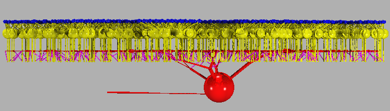
|
An experiment in retsim consists of function calls to the Neuron-C library. These functions (the NeuronC API) are defined in "nc/src/ncfuncs.h" and described in the NeuronC User's Manual. Each function call in "ncfuncs.h" replaces a statement in the interpreted version of NeuronC. The retsim script defines an array of neurons and connects them using these function calls. To see an example of source code for this compiled version, see the "retsim.cc" model in nc/models/retsim". The command-line switches for "retsim" are identical to those listed by "nc -h", but note that running "retsim" without arguments displays a list of simulation experiments and parameters. In addition simulation variables can be set from the command line.
The NeuronC API is incorporated into a static library called "libnc.a". This file is created in "nc/src" and must be linked with a neural circuit program such as "nc/models/retsim/retsim.cc". To link this library correctly you may need to set the "NC_HOME" variable in nc/models/retsim/makefile, either by setting it as an environment variable or by changing the makefile. The libnc.a library is created as a static library because as a dynamic library it reduces run-time speed.
The experiments defined for "nc/models/retsim" such as "expt_gc_cbp_flash.cc" are compiled to be dynamically linked to the "retsim" program at runtime, i.e. each experiment is compiled into a dynamic library, e.g. "expt_gc_cbp_flash.so". To allow this process of dynamic runtime linking, you must set the environment variable LD_LIBRARY_PATH or include the directory where the experiment ".so" file is located in (for Linux) "/etc/ld.so.conf". That will allow the runtime linker to find "expt_gc_cbp_flash.so"
(if using tcsh)  setenv LD_LIBRARY_PATH .            [[ place in your ~/.cshrc file ]]
(if using bash)  export LD_LIBRARY_PATH="."          [[ place in your ~/.profile file ]]
Another way to direct the dynamic linking process is to make a symbolic link from a file in /usr/local/lib to the experiment .so file in nc/models/retsim. The dynamic linker will identify the file because it starts with "lib_":
ln -s /usr/local/lib/lib_expt_gc_cbp_flash.so expt_gc_cbp_flash.so
At the top of the "retsim.cc" script, several files are included:
 #include "ncio.h"         // defines "ncfprintf()" for I/O to a C++ stream
 #include "ncfuncs.h"      // defines the C++ functions for the simulator
 #include "retcolors.h"    // defines the standard colors 0-15
 #include "retsim.h"       // defines constants and functions for retsim.cc
 #include "retsim_var.cc"  // defines parameters and "setptrs()" which initializes them
 #include "ncinit.h"       // defines a null "setptrs()" in case it is not already defined
 #include "setexpt.h"      // defines "defparams()", "setparams()", "setdens()", "addcells()",
			   //    "addsyns()", "addlabels()" and "runexpt()" for the experiment file
Most of these header files are in the retsim directory, but some are in the nc/src directory. If you are compiling retsim in a different location than nc/models/retsim, you need to set the NC_HOME environment variable in "retsim/makefile":
# NC_HOME = ~/nc
For some of the old Mac compilers, the -O and -O3 optimizations caused retsim to crash. You may need to remove the optimizations defined by CFLAGS at the top of nc/src/makefile:
cd nc/srcChange this (lines 1-2, nc/src/makefile):
CFLAGS = -O3
# CFLAGS =      # for Mac OSX
to this:
# CFLAGS = -O3
CFLAGS =      # for Mac OSX
Then (in nc/src):
make
When compiling retsim (see "Retsim: a retinal simulator" in ncman6.html), you will also have to modify the makefile for retsim's dynamic linking. The Mac OSX uses a slightly different way to link dynamic libraries. From the nc/models/retsim directory, you need to edit the "makefile" which is responsible for compiling and linking retsim. You only need to uncomment the line (i.e. remove the "#"):
cd ~/nc/models/retsimChange this (line 1, nc/src/retsim/makefile):
CFLAGS = -Ofastto this:
# CFLAGS = -OfastChange this (line 6, nc/src/retsim/makefile):
# CFLAGS = # for Mac OSXto this:
CFLAGS = # for Mac OSXChange this (line 47, nc/src/retsim/makefile)
# OSFLAGS = -DMACOSXto this:
OSFLAGS = -DMACOSX
After you've modified the makefiles, then enter "make" on the command line. If you need to modify nc/src/makefile, you'll need to run make there, too. This will compile and link all the source code correctly on the Mac. For this to work, you will need to have XCode (the C compiler) installed.
CFLAGS = -OfastUncomment the line:
# CFLAGS = -Ofast -fPIC # for 64-bit systemsso it looks like this:
# CFLAGS = -Ofast
CFLAGS = -Ofast -fPIC  # for 64-bit systems
For Mac OSX systems you don't need to uncomment the -Ofast -fPIC lines.
Normally, the command line parameters are automatically converted into numeric values when the first charater of the command line value is numeric. This is usually what is desired, and the "setptr()" function sets the type correctly according to the variable type in its definition. However, if you want to allow a string parameter to accept a numeric value, you can do this with the "setvarstr(char *)" function, calling it with the parameter's name after the command line has been read and converted. This function retrieves the original character string from the command line that was associated with the parameter name, and loads this char string into the "char *parameter" after the command line has been converted.
Command line that accepts a text or numeric value for filename:
retsim --expt ... --filename xxx // first char of xxx can be text or numericin the expt file:
char *filename;in "defparams()":
setptr("filename", &filename);
in "setparams()":
setvarstr("filename")
if (notinit(filename)) filename = "yyy";
  void runexpt(void)
  {
    double Vmin, Vmax;
    ...
    if (notinit(prestimdur))    prestimdur =  0.02;      /* sets default timing, override on command line
    if (notinit(poststimdur))  poststimdur =  0.05;
    if (notinit(tailcurdur))    tailcurdur =  0.02;
    ...
    plot_i_nod(ct=gca,cn=1,n=soma,Vmin=-.067,Vmax =-.027,colr=cyan,"", -1, -1); /* plot soma current*/
    ...

    sprintf (savefile,"vclamp_save%06d",getpid());       /* add process id to save file name */
    savemodel (savefile);				 /* make a save file to save simulation state
    if (vstart < vstop) sign = 1;
    else                sign = -1;
    for (i=0,vpulse=vstart; (vpulse*sign)<=(vstop*sign+1e-6); i++,vpulse += vstep) {
        simtime = 0;					/* set the simulation time back to zero */
        pulsedur = move_stim(stimtime, ...);		/* run the stimulus */
        vclamp (ndn(ct,cn, soma), vhold, simtime,  prestimdur);       /* clamp to vhold */
        vclamp (ndn(ct,cn, soma), vpulse, simtime,  pulsedur);        /* clamp to the pulse voltage */
        vclamp (ndn(ct,cn, soma), tailvolt, simtime,  tailcurdur);    /* look at the tail currents */
        vclamp (ndn(ct,cn, soma), vhold, simtime, poststimdur);       /* return to vhold */
        restoremodel (savefile);				      /* restore all states to before vclamp */
    }
    unlink (savefile);						      /* remove the save file */
  }
Note that the variables tested by notinit() must be defined in "defparams()" in
order to be set from the command line.
   retsim --expt gc_cbp_flash --ninfo 2 -d 1 -v                      | vid

   retsim --expt gc_cbp_flash --ninfo 2 | less                                    # quit from less with "q"

   retsim --expt gc_cbp_flash --ninfo 2 --node_scale -3.05 -d 9 -v   | vid

   retsim --expt gc_cbp_flash --ninfo 2 -d 9 -v                      | vid -c > file.ps  #  make .ps file.

   retsim --expt gc_cbp_flash -d 1 -R           > file.pov

   povray +h1000 +w1000 +ifile.pov +dx                                              #  generate image with povray

   retsim --expt gc_cbp_flash --mxrot 90 -d 1 -v                     | vid

   retsim --expt gc_cbp_flash --flip 1 -d 1 -v                       | vid

   retsim --expt gc_cbp_flash --ninfo 2 --arrsiz 100 -d 1 -v         | vid

   retsim --expt gc_cbp_flash --ninfo 2 --n_cbp 1 --n_gc 0 -d 1 -v   | vid

   retsim --expt gc_cbp_flash --ninfo 2 -v                           | vid

   retsim --expt gc_cbp_flash           > file.r

   plotmod file.r | vid                                                             #   display plots from data file
For csh/tcsh shell:

retsim --expt ... --ninfo 2 ... > file.r           [only the stdout (data) stream goes into the file]
retsim --expt ... --ninfo 0 ... > file.r           [no connection info printed, only the stdout stream goes into the file]
retsim --expt ... --ninfo 2 ... >& file.r          [both stdout and stderr streams go into the file]
Adding a second & after the file name runs the command in the background:
retsim --expt ... --ninfo 2 ... >& file.r &


For some versions of the bash shell, you may need to change ">&" to "2>&1 >":

retsim --expt ... --ninfo 2 ... 2>&1 > file.r     [both stdout and stderr streams go into the file]
Plot functions defined in "plot_funcs.cc" and "retsim.h": plot_v_nod() Plots voltage at a node. Can be combined with searches for nodes by location. plot_i_nod() Plots current at a node. Can be combined with searches for nodes by location. plot_l_nod() Plots light flux at a node. Can be combined with searches for nodes by location. plot_ca_nod() Plots calcium conc at a node. Can be combined with searches for nodes by location. plot_ca_syn() Plots calcium conc at a synapse. Can be combined with searches for nodes by location. plot_spike_rate() Plots instantaneous spike rate as color of point. plot_chan() Plots channel conductance or the population of any Markov state plot_chan_cond() Plots channel conductance, can be combined with searches for nodes by location. plot_chan_current() Plots channel current, can be combined with searches for nodes by location. plot_synrate() Plots synaptic release, including vesicle release rate, vesicles, and postsynaptic conductance. void plot_l_nod(int ct,int cn, int n, double lmin, double lmax,int pcolor,const char *label, int plotnum, double psize); void plot_v_nod(int ct,int cn, int n, double vmin, double vmax,int pcolor,const char *label, int plotnum, double psize); void plot_v_nod(node *npnt, double vmin, double vmax,int pcolor,const char *label, int plotnum, double psize); void plot_i_nod(int ct,int cn, int n, double vmin, double vmax,int pcolor,const char *label, int plotnum, double psize); void plot_ca_nod(int ct, int cn, int n,double maxca, int pcolor, const char *label, int plotnum, double psize); void plot_ca_nod(int ct, int cn, int n, int sh, double maxca, int pcolor, const char *label, int plotnum, double psize); void plot_ca_nod(node *n, int sh, double maxca, int pcolor, const char *label, int plotnum, double psize); void plot_ca_syn(synapse *s, int sh, double maxca, int pcolor, const char *label, int plotnum, double psize); void plot_ca_syn(synapse *s, double maxca, int pcolor, const char *label, int plotnum, double psize); void plot_cabufb_nod(int ct, int cn, int n,double maxca, int pcolor, const char *label, int plotnum, double psize); void plot_cabufb_nod(int ct, int cn, int n, int sh, double maxca, int pcolor, const char *label, int plotnum, double psize); void plot_ph_nod(node *npnt, double maxnt, double minnt, int pcolor, const char *label, int plotnum, double psize); void plot_ph_nod(int ct, int cn, int n, double maxnt, double minnt, int pcolor, const char *label, int plotnum, double psize); Functions to add synapse to list(s) of synapses for run time recording, analysis, and display: int synapse_add (int synlist, int ct, int cn, int nod, int ct2, int cn2); int synapse_add (int synlist, int ct, int cn, int nod, int ct2, int cn2, double vrev); int synapse_add (int synlist, int ct, int cn, int nod, int ct2, int cn2, int connum); Functions to plot parameters from lists of synapses (defined by "synapse_add()" above): double rsyn_avg (double sl, double time); Plot average rate of list of synapses double isyn_avg (double sl, double time); Plot average current of list of synapses double isyn_tot (double sl, double time); Plot average conductance of list of synapses double gsyn_avg (double sl, double time); Plot total current of list of synapses double gsyn_tot (double sl, double time); Plot total conductance of list of synapses double gnmda_syn_tot (double sl, double time); Plot total conductance of list of NMDA synapses Functions to plot synaptic parameters, using different combinations of arguments: void plot_synrate(int ct, int cn, int nod, int prate, double rmin, double rmax, int pves, double fmin, double fmax, int pcond, double cmin, double cmax, int pcolor, int plotnum, const char *plname, double plsize); void plot_synrate(int ct, int cn, int nod, double rmin, double rmax, int pcolor, int plotnum, const char *plname, double plsize); void plot_synrate(int ct, int cn, int prate, double rmin, double rmax, int pves, double fmin, double fmax, int pcond, double cmin, double cmax, int pcolor, int plotnum, const char *plname, double plsize); void plot_synrate(int ct, int cn, int prate, double rmin, double rmax, int pves, double fmin, double fmax, int pcolor, int plotnum, const char *plname, double plsize); void plot_synrate(int ct, int cn, double rmin, double rmax, int pcolor, int plotnum, const char *plname, double plsize); void plot_synves (int ct, int cn, int ves, double fmin, double mmax, int pcolor, int plotnum, const char *plname, double plsize); void plot_synves (int ct, int cn, double fmin, double mmax, int pcolor, int plotnum, const char *plname, double plsize); void plot_syncond(int ct, int cn, int nod, double cmin, double cmax, int pcolor, int plotnum, const char *plname, double plsize); void plot_mglur2 (int ct, int cn, int nod, double mmin, double mmax, int pcolor, int plotnum, const char *plname, double plsize); void plot_mglur2 (int ct, int cn, double mmin, double mmax, int pcolor, int plotnum, const char *plname, double plsize); void plot_mglur2p(int ct, int cn, double mmin, double mmax, int pcolor, int plotnum, const char *plname, double plsize); void plot_syncond(int ct, int cn, double cmin, double cmax, int pcolor, int plotnum, const char *plname, double plsize); void plot_synrate(synapse *s, int prate, double rmin, double rmax, int pves, double fmin, double fmax, int pcond, double cmin, double cmax, int pcolor, int plotnum, const char *plname, double plsize); void plot_synrate(synapse *s, double rmin, double rmax, int pcolor, int plotnum, const char *plname, double plsize); void plot_syncond(synapse *s, double cmin, double cmax, int pcolor, int plotnum, const char *plname, double plsize); void plot_syncondp(synapse *s, double cmin, double cmax, int pcolor, int plotnum, const char *plname, double plsize); void plot_synves(synapse *s, double cmin, double cmax, int pcolor, int plotnum, const char *plname, double plsize); void plot_mglur2(synapse *s, double mmin, double mmax, int pcolor, int plotnum, const char *plname, double plsize); Functions to plot output synaptic rate, using different combinations of arguments: void plot_synrate_out(int ct, int cn, double rmin, double rmax, int colr); void plot_synrate_out(int ct, int cn, double rmin, double rmax, int colr, const char *plname); void plot_synrate_out(int ct, int cn, double rmin, double rmax, int colr, double plsize); void plot_synrate_out(int ct, int cn, double rmin, double rmax, int colr, const char *plname, double plsize); void plot_synrate_out(int ct, int cn, int ct2, int cn2, double rmin, double rmax, int colr, int prate); void plot_synrate_out(int ct, int cn, int ct2, int cn2, double rmin, double rmax, int colr, int prate, const char *plname); void plot_synrate_out(int ct, int cn, int ct2, int cn2, double rmin, double rmax, int colr, int prate, double plsize); void plot_synrate_out(int ct, int cn, int ct2, int cn2, double rmin, double rmax, int colr, int prate, const char *plname, double plsize); void plot_synrate_out(int ct, int cn, int ct2, int cn2, double rmin, double rmax, double fmax, int colr, int prate); void plot_synrate_out(int ct, int cn, int ct2, int cn2, double rmin, double rmax, double fmax, int colr, int prate, const char *plname); void plot_synrate_out(int ct, int cn, int ct2, int cn2, double rmin, double rmax, double fmax, int colr, int prate, double plsize); void plot_synrate_out(int ct, int cn, int ct2, int cn2, double rmin, double rmax, double fmax, int colr, int prate, const char *plname, double plsize); void plot_synrate_out(int ct, int cn, int nod, int ct2, int cn2, double rmin, double rmax, int colr,int prate); void plot_synrate_out(int ct, int cn, int nod, int ct2, int cn2, double rmin, double rmax, int colr,int prate, const char *plname); void plot_synrate_out(int ct, int cn, int nod, int ct2, int cn2, double rmin, double rmax, int colr,int prate, int pves, double plsize); void plot_synrate_out(int ct, int cn, int nod, int ct2, int cn2, double rmin, double rmax, int colr,int prate, int pves, const char *plname, double plsize); void plot_synrate_out(int ct, int cn, int nod, int ct2, int cn2, double rmin, double rmax, double fmax, int colr,int prate); void plot_synrate_out(int ct, int cn, int nod, int ct2, int cn2, double rmin, double rmax, double fmax, int colr,int prate, const char *plname); void plot_synrate_out(int ct, int cn, int nod, int ct2, int cn2, double rmin, double rmax, double fmax, int colr,int prate, int pves, double plsize); void plot_synrate_out(int ct, int cn, int nod, int ct2, int cn2, double rmin, double rmax, double fmax, int colr,int prate, int pves, const char *plname, double plsize); Functions to plot channel parameters: void plot_spike_rate(int ct, int cn, int n, int pcolor, const char *label, int plotnum, double psize); void plot_chan(int ct, int cn, int n, int ctype, int stype, int param, double pmax, double pmin); void plot_chan(int ct, int cn, int n, int ctype, int stype, int param, int pval, double pmax, double pmin); void plot_chan_current(int ct, int cn, int n, int ctype, int stype, double pmax, double pmin); void plot_chan_current(int ct, int cn, int n, int ctype, int stype, double mult, double pmax, double pmin); void plot_chan_cond(int ct, int cn, int n, int ctype, int stype, double pmax, double pmin); void plot_chan_cond(int ct, int cn, int n, int ctype, int stype, double mult, double pmax, double pmin); void plot_chan_state(int ct, int cn, int n, int ctype, int stype, int param, double pmax, double pmin, const char *label, int plotnum, double psize); Example: plot_chan(ct=dbp1, cn=1, dend_node, CGMP, 1, G, state=1, pmax=2, pmin=0); Plot functions in "ncfuncs.cc" (defined in ncfuncs.h): plot (V,); plot (V, , max= , min= ); plot (I, ); plot (L, ); plot (V, ); plot (FAn, n, , max= , min= ); plot (FBn, n, , max= , min= ); plot (FCn, n, , max= , min= ); plot (Ca, n, , max= , min= ); plot (G, n, , max= , min= ); plot_var Plots value of variable at run time plot_func() Plots value returned by function at run time Misc functions defined in "celfuncs.cc" and "retsim.h": round() Rounds up a floating point number to the nearest integer modangl() Converts angle to range 0 - 2PI sindeg() Sine function in degrees cosdeg() Cosine function in degrees atanx() Similar to atan2(y,x) function in the C library inrange() Determines whether number is within a range rrange() Returns random number within a range mid() Returns middle element in array midrow() Returns start of middle row of array ff() Returns 1 or -1 with 50% chance gauss() Returns gaussian function node_angle() Returns angle between 2 nodes get_angles() Calculates average orientation angle of dendrite rad_dist() Computes distance from node along dendrite to soma rad_dir() Determines which node of a cable segment is closest to the soma taperden() Makes tapered dendrite taperdistden() Makes tapered dendrite, starting from existing dendrite taperdia() Finds diameter of distal dendrite sigm() Returns y-val on specified sigmoidal function comp_phase() Computes phase for a sine wave with a specified delay time sinewaves() Adds 2 sine waves, returns sum makanatfile() Makes an anatomy file out of an existing artificial cell morphology dendn_node() Look up number in dendn column of morph file, return its node number Misc functions defined in "synfuncs.cc" and "retsim.h": print_connections() Print connections for all cells of a given type. print_avg_connections() Print the average number of connections to other types ncel_in() Return number of presynaptic cells of a given type to a specific cell tot_ncel_in() Return total number of presynaptic cells to a specific cell tot_ncel_ind() Return total number of presynaptic cells of a different type to a specific cell ncel_out() Return number of postsynaptic cells of a given type to a specific cell tot_ncel_out() Return total number of postsynaptic cells to a specific cell tot_ncel_outd() Return total number of postsynaptic cells of a different type to a specific cell connected() Determine whether a cell is synaptically connected to another connected2() Determine whether a cell synaptically converges from a second to a third type connected3() Determine whether a cell converges from a second to a third type Functions to find cells and nodes within cells: findmid() Finds middle cell in array, useful for recording findmida() Finds cell closest to x,y offset in array, useful for recording findmidc() Finds middle cell by count findnodloc() Finds node closest to x,y offset in celltype, cellnum. Maxdist is optional findnodlocr() Finds node closest to x,y offset from soma of celltype, cellnum. Maxdist is optional findnodlocz() Finds node closest to x,y offset of celltype, within z range int findmid(int ct, double xoffset, double yoffset); int findmida(int ct, double xoffset, double yoffset); int findnodloc(int ct, int cn, double xoffset, double yoffset); int findnodloc(int ct, int cn, double xoffset, double yoffset, double maxdist); int findnodlocr(int ct, int cn, double xoffset, double yoffset); int findnodlocr(int ct, int cn, double xoffset, double yoffset, double maxdist); int findnodlocra(int ct, int cn, double roffset, double theta); int findnodlocra(int ct, int cn, double roffset, double theta, double maxdist); int findnodlocz(int ct, int cn, double xoffset, double yoffset,double zmax, double zmin); findsynloc() Finds synapse at node closest to x,y offset of celltype, cellnum is optional findsynlocr() Finds synapse at node closest to x,y offset from soma of celltype, cellnum, vrev, maxdist are optional, second cell of celltype2, cellnum2 is optional Functions to find a synapse by cell and location: synapse *findsynloc(int ct, double xoffset, double yoffset); synapse *findsynloc(int ct, int cn, double xoffset, double yoffset); synapse *findsynloc(int ct, int cn, double xoffset, double yoffset, double vrev); synapse *findsynloc(int ct, int cn, double xoffset, double yoffset, double vrev, double maxdist); synapse *findsynloc(int ct, int cn, int ct2, int cn2, double xoffset, double yoffset, double vrev); synapse *findsynloc(int ct, int cn, int ct2, int cn2, double xoffset, double yoffset, double vrev, double maxdist); Find by direction from center of array: synapse *findsynloca(int ct, double roffset, double theta); synapse *findsynloca(int ct, int cn, double roffset, double theta); Find by distance from soma: synapse *findsynlocr(int ct, int cn, double xoffset, double yoffset); synapse *findsynlocr(int ct, int cn, double xoffset, double yoffset, double vrev); synapse *findsynlocr(int ct, int cn, int ct2, int cn2, double xoffset, double yoffset, double vrev); synapse *findsynlocr(int ct, int cn, int ct2, int cn2, double xoffset, double yoffset, double vrev, double maxdist); Find by radius, theta from soma: synapse *findsynlocra(int ct, int cn, double roffset, double theta); synapse *findsynlocra(int ct, int cn, double roffset, double theta, double vrev); synapse *findsynlocra(int ct, int cn, int ct2, int cn2, double roffset, double theta, double vrev); synapse *findsynlocra(int ct, int cn, int ct2, int cn2, double roffset, double theta, double vrev, double maxdist); int findsynlocx(int ct, int cn, double xoffset, double yoffset); find_maxmin() Calculates max,min in x,y of complete array, celltype and cellnum are optional find_maxrad() Calculates max radius of complete array, celltype and cellnum are optional Stimulus functions for retsim, defined in stimfuncs.cc and stimfuncs.h:
double movebar(double starttime, double xcent, double ycent, double r1, double r2, double bwidth, double blength, double theta, double velocity, double sinten); double movebar(double starttime, double xcent, double ycent, double r1, double r2, double bwidth, double theta, double velocity, double sinten); double stepspot(double starttime,double x1,double x2,double y,double bdia, double velocity, double sinten); double moveannulus(double starttime,double xcent, double ycent, double r1,double r2, double anndia, double velocity, double sinten); void movesineann (double x,double y,int direction,double ann_gaussenv,double centdia, double phase,double speriod, double stfreq,double sinten, double contrast,int sq, double starttime,double sdur); void movewindmill (double x, double y, int direction, double ann_gaussenv,double centdia, double phase, double speriod, double stfreq, double sinten, double scontr, int sq, double starttime, double sdur); double twospot(double starttime, double xcent, double ycent, double r1, double r2, double dia, double theta, double sinten, double dur, double timestep); void square_wave_i (node *nd, double freq, double i, double start, double dur); void sine_wave_i (node *nd, double freq, double i, double start, double dur, double tstep); void ramp_c (node *nd, double cstart, double cstop, double start, double dur, double tstep); void ramp_v (node *nd, double vstart, double vstop, double start, double dur, double tstep);
Standard stimulus functions in nc, defined in ncfuncs.h (ncstimfuncs.cc):
void stim_node (node *npnt, double inten, double start, double dur, double wavel); void stim_node (node *npnt, double inten, double start, double dur); void stim_cone (node *npnt, double inten, double start, double dur, double wavel); void stim_cone (node *npnt, double inten, double start, double dur); void stim_rod (node *npnt, double inten, double start, double dur, double wavel); void stim_rod (node *npnt, double inten, double start, double dur); void stim_bar (double width, double length, double xloc, double yloc, double xcent, double ycent, double scale, double orient, double inten, double start, double dur, double wavel, double mask); void stim_bar (double width, double length, double xloc, double yloc, double orient, double inten, double start, double dur, double wavel, double mask); void stim_bar (double width, double length, double xloc, double yloc, double orient, double inten, double start, double dur); void stim_spot (double dia, double xloc, double yloc, double xcent, double ycent, double scale, double inten, double start, double dur, double wavel, double mask); void stim_spot (double dia, double xloc, double yloc, double inten, double start, double dur, double wavel, double mask); void stim_spot (double dia, double xloc, double yloc, double inten, double start, double dur); void stim_ispot (double dia, double xloc, double yloc, double inten, double start, double dur, double wavel, double mask, int invert); void stim_grating (int type, double speriod, double sphase, double orient, double xloc, double yloc, double tfreq, double drift, double inten, double contrast, double wavel, double xenv, double yenv, double mask, double start, double dur); void stim_sine(double speriod, double sphase, double orient, double xloc, double yloc, double xcent, double ycent, double tfreq, int drift, double scale, double inten, double contrast, double start, double dur, double wavel, double mask); void stim_sine(double speriod, double sphase, double orient, double xloc, double yloc, double tfreq, int drift, double inten, double contrast, double start, double dur); void stim_gabor(double speriod, double sphase, double orient, double xloc, double yloc, double xcent, double ycent, double tfreq, double drift, double scale, double inten, double contrast, double xenv, double yenv, int sq, double start, double dur, double wavel, double mask); void stim_gabor(double speriod, double sphase, double orient, double xloc, double yloc, double tfreq, double drift, double inten, double contrast, double xenv, double yenv, int sq, double start, double dur); void stim_sineann(double speriod, double sphase, double xloc, double yloc, double xcent, double ycent, double tfreq, double drift, double scale, double inten, double contrast, double xenv, int sq, double start, double dur, double wavel, double mask); void stim_sineann(double speriod, double sphase, double xloc, double yloc, double tfreq, double drift, double inten, double contrast, double xenv, double start, double dur); void stim_sineann(double speriod, double sphase, double xloc, double yloc, double tfreq, double drift, double inten, double contrast, double xenv, int sq, double start, double dur); void stim_windmill(double speriod, double sphase, double xloc, double yloc, double xcent, double ycent, double tfreq, double drift, double scale, double inten, double contrast, double xenv, int sq, double start, double dur, double wavel, double mask); void stim_windmill(double speriod, double sphase, double xloc, double yloc, double tfreq, double drift, double inten, double contrast, double xenv, double start, double dur); void stim_windmill(double speriod, double sphase, double xloc, double yloc, double tfreq, double drift, double inten, double contrast, double xenv, int sq, double start, double dur); void stim_checkerboard(double width, double height, int xn, int yn, double orient, double xloc, double yloc, double xcent, double ycent, double scale, double tfreq, double inten, double contrast, double start, double dur, double **stim_rndarr, int *stim_nfr); void stim_checkerboard(double width, double height, int xn, int yn, double orient, double xloc, double yloc, double tfreq, double inten, double contrast, double start, double dur,double **stim_rndarr, int *stim_nfr); void stim_file (const char *filename); void stim_backgr (double backgr, double wavel, double mask, double start); void stim_backgr (double backgr, double start); void stim_backgr (double backgr); void vclamp (node *npnt, double inten, double start, double dur); void cclamp (node *npnt, double inten, double start, double dur); void puff (node *npnt, int puffmsg, double inten, double start, double dur);
expt_aii_dbp.cc               Make a bipolar cell and run voltage-clamp
expt_cbp_vclamp.cc            Voltage-clamp a bipolar cell
expt_cbp_cclamp.cc            Current-clamp a bipolar cell
expt_aii_flash.cc             Make an AII amacrine, RBPs, and rods with light stim
expt_cbp_feedback.c           Make a bipolar cell with amacrine feedback
expt_cbp_flash.cc             Make a bipolar cell with light stim
expt_cell_vclamp.cc           Voltage-clamp a cell
expt_cone_hz.cc               Construct cone-horizontal cell circuit and run voltage clamp
expt_cone_hz_cvc.cc           Construct cone-horizontal cell circuit and run voltage clamp
expt_cone_hz_hvc.cc           Construct cone-horizontal cell circuit and run voltage clamp
expt_dsgc_calib.cc            Voltage clamp a cell
expt_dsgc_cbp_bar.cc          Construct a bipolar cell and stimulate with light bar
expt_dsgc_cbp_stim.cc         Construct a bipolar cell and stimulate with light
expt_dsgc_cbp_twospot.cc      Construct a bipolar cell and stimulate with spots
expt_dsgc_chans.cc            Voltage clamp a DS ganglion cell
expt_dsgc_pair.cc             Voltage clamp 2 DSGCs, one with chans and other without, subtract
expt_dsgc_sbac_bar.cc         Construct DSGC with SB amacrine, stimulate with light bar
expt_gc_Rin.cc                Compute Rin for ganglion cell
expt_gc_cbp_flash.cc          Construct On ganglion cell and its feedforward cone bipolar circuit
expt_gc_bphz_flash.cc         Construct On ganglion cell and its presynaptic cone bipolar circuit
expt_gc_cbp_aii_flash.cc      Construct On ganglion cell and its bipolar and AII amacrine circuit
expt_gc_cbp_am_flash.cc       Construct On ganglion cell with bipolar cells and amacrine feedback
expt_gcoff_hbp_flash.cc       Construct Off ganglion cell and its feedforward cone bipolar circuit
expt_gcoff_hbp_flashes.cc     Construct Off ganglion cell and its feedforward cone bipolar circuit
expt_gcoff_hbp_flicker.cc     Stimulate Off ganglion cell circuit with flickering spot
expt_rbp_aii_a17.cc           Construct rod bipolar connected to AII and A17 amacrines
expt_sbac_stim.cc             Construct arrays of SB amacrine cells and stimulate with moving bar
expt_sbac_vclamp.cc           Voltage-clamp a SB amacrine cell
expt_wfamac.cc                Make a wide-field amacrine cell

expt_cell_Rin.cc              Make a cell from a morphology file and measure Rin (temporal)
expt_surf_area.c              Make a cell from a morphology file and measure surface area, Rin (static)
expt_morph_props.cc           Make a cell from a morphology file and display morphological props
expt_test.cc                  Very simple test file to start an experiment
A useful experiment is "expt_surf_area.cc".
# surface area and conductances
#
retsim --expt surf_area --celltype dsgc --n_dsgc 1 --dsgc_file morph_ds1e --dsgc_densfile dens_dsgc.n
       --nvalfile nval_dsgc_sbac.n --dvrev -0.06 --dvst -0.06 --drm 10e3 --dendrm 35e3 --dri 200
       --ninfo 2 > dsgc_surf_area.txt
This command gives the printout:
# Retina simulation
#
#   retsim version:    1.7.56
#   nc version:        6.2.15
#   date:              Fri Jan 30 16:30:00 EST 2015
#   machine:           bip
#   experiment:        surf_area
#   confdir:           runconf
#   nvalfile:          nval_dsgc_sbac.n
#   dsgc  morph:       morph_ds1e,   densities: dens_dsgc.n
#   chanparams file:   chanparams
#
#c 3315 neural elements (21.6 MB) converted to compartments.
#c 3315 neural elements saved.
#c Total memory space used 24.3 MB.
#c 453 comps, 3287 nodes, 452 connections, 2532 channels.
#
# Surface area and conductances of dsgc
#
# nval file          nval_dsgc_sbac.n
# density file       dens_dsgc.n
#
# Region   R12       R15       R16       R17       R18       R19       Tot
# Label    DendD     Soma      HCK       AxonT     AxonP     AxonD     Cell
# color    blue      red       blue      cyan      magenta   green
#
# Area     1.464e+04 917.6     5.235     34.59     1475      7689      2.476e+04 um2
# CompLam  0.1       0.2       0.1       0.1       0.1       0.1                 Lambda/comp
#
# Rm       1e+04     1e+04     1e+04     1e+04     1e+04     1e+04     1e+04     Ohm-cm2
# Ri       200       200       200       200       200       200                 Ohm-cm
# Cm       1         1         1         1         1         1                   uF/cm2
#
# Rin      68.3      1.09e+03  1.91e+05  2.89e+04  678       130       40.39     MOhm (from Rm only)
# Cond     1.464e+04 917.6     5.235     34.59     1475      7689      2.476e+04 pS   (from Rm only)
# Cm       146.4     9.176     0.05235   0.3459    14.75     76.89     247.6     pF
# Cond/cap 100       100       100       100       100       100       100       pS/pF
#
# NA2      0         0         0         0         50        50        18.51     mS/cm2
# NA6      35        4         4         100       0         0         20.98     mS/cm2
# K1       15        15        15        20        10        10        13.16     mS/cm2
# K3       35        35        35        0         0         0         22        mS/cm2
# K4       0         0.09      0         0.8       0.8       0         0.05211   mS/cm2
# KCA4     0.12      0.12      0         0         0         0         0.07539   mS/cm2
# KCA5     0.01      0.04      0.02      0         0         0         0.007399  mS/cm2
# CA0      0.014     0.014     0.014     0         0         0         0.008799  mS/cm2
#
# NA2      0         0         0         0         737.5     3845      4582      nS
# NA6      5123      36.7      0.2094    34.59     0         0         5195      nS
# K1       2196      137.6     0.7853    6.917     147.5     768.9     3258      nS
# K3       5123      321.1     1.832     0         0         0         5446      nS
# K4       0         0.8258    0         0.2767    11.8      0         12.9      nS
# KCA4     17.57     1.101     0         0         0         0         18.67     nS
# KCA5     1.464     0.367     0.001047  0         0         0         1.832     nS
# CA0      2.049     0.1285    0.000733  0         0         0         2.179     nS
For each region of the cell, the printout gives several types of information: the surface area, the compartment size "complam", the Rm, Ri, and Cm, the input resistance Rin and the conductance calculated from Rm, the capacitance h, and the ratio of conductance/capacitance. It also gives the channel densities for all of the channel types defined in the density file.
Another experiment is "expt_gc_cbp_flash.cc". To make a display of the model:
retsim --expt gc_cbp_flash -d 1 -v | vidTo run the experiment:
 retsim --expt gc_cbp_flash -v | vid
or:
 retsim --expt gc_cbp_flash  > gc_cbp_flash.r
 plotmod gc_cbp_flash.r | vid
or:
 retsim --expt gc_cbp_flash --temp_freq 4 --ntrials 40 --dstim 0.1 --sdia 100
           --scontrast 0.8 > gc_cbp_flash_n40.d100.c0.8.r
The experiment:
/* Experiment gc_cbp_flash */ /* for nc script retsim.cc */ #include#include #include #include "ncfuncs.h" #include "retsim.h" #include "retsim_var.h" double temp_freq; double ntrials; double dstim; double sdia; double stimtime; double minten; double scontrast; double setploti; int rec_ct; int rec_cn; /*------------------------------------------------------*/ void defparams(void) { setptr("temp_freq", &temp_freq); setptr("ntrials", &ntrials); setptr("dstim", &dstim); setptr("sdia", &sdia); setptr("stimtime", &stimtime); setptr("minten", &minten); setptr("scontrast", &scontrast); setptr("setploti", &setploti); nvalfile = "nval_gc_cbp_flash.n"; } /*------------------------------------------------------*/ void setparams(void) { make_rods = 0; make_cones= 1; /* make cones, dbp, gc */ make_ha = 0; make_hb = 0; make_hbat = 0; make_dbp1 = 1; make_dbp2 = 0; make_rbp = 0; make_gca = 1; make_gcb = 0; make_dsgc = 0; if(notinit(rec_ct)) rec_ct = gca; //if (notinit(arrsiz)) arrsiz = 300; if (notinit(bg_inten)) bg_inten = 2.0e4; /* background light intensity */ //if (arrsiz==100) { // setsv (dbp1,SCOND,1, 25e-10); //} } /*------------------------------------------------------*/ void runexpt(void) { int ct, cn, n, plnum; int colr; int midcone, midcbp, midcbp2; int synin1, synin2; double t, fmax,fmin; double rmin, rmax, plsize; double dtrial,exptdur; double Vmin, Vmax; if (notinit(temp_freq)) temp_freq = 2; if (notinit(ntrials)) ntrials = 1; if (temp_freq == 0) { fprintf (stderr,"## retsim1: temp_freq = 0, STOPPING\n"); temp_freq = 1; }; dtrial = 1 / temp_freq; exptdur = dtrial * ntrials; endexp = exptdur; ploti = 1e-4; if (notinit(dstim)) dstim = .05; /* stimulus duration */ if (notinit(sdia)) sdia = 300; /* spot diameter */ if (notinit(stimtime)) stimtime = .10; /* stimulus time */ if (notinit(minten)) minten = bg_inten; /* background intensity (for make cone)*/ if (notinit(scontrast)) scontrast = .5; /* intensity increment */ if (!notinit(setploti)) ploti = setploti; /* plot time increment */ midcone = findmid(xcone,0,0); midcbp = findmid(dbp1,0,0); midcbp2 = findmid(dbp1,10,10); //midcbp2 = find_gtconn(dbp1, 8); synin1 = ncel_in(dbp1,midcbp,xcone); synin2 = ncel_in(dbp1,midcbp2,xcone); if (ninfo >=1) fprintf (stderr,"# mid cone # %d\n", midcone); if (ninfo >=1) fprintf (stderr,"# mid cbp # %d ncones %d\n", midcbp,synin1); if (ninfo >=1) fprintf (stderr,"# mid cbp2 # %d ncones %d\n", midcbp2,synin2); plot_v_nod(ct=xcone,cn=midcone,n=soma,Vmin=-.030,Vmax =-.025,colr=cyan,"", -1, -1); /* plot Vcones*/ plot_synrate_out(ct=xcone,cn=midcone,rmin=0,rmax=400,colr=magenta); /* plot rate out */ plot_v_nod(ct=dbp1,cn=midcbp,n=soma, Vmin=-.045,Vmax =-.035,colr=red,"", -1, -1); /* plot Vcbp */ plot_v_nod(ct=dbp1,cn=midcbp2,n=soma,Vmin=-.045,Vmax =-.035,colr=green,"", -1, -1); /* plot Vcbp */ plot_synrate_out(ct=dbp1,cn=midcbp,rmin=0,rmax=200,colr=magenta); /* plot rate out */ plot_v_nod(ct=gca, cn=1,n=soma,Vmin=-.070,Vmax =-.050,colr=blue,"", -1, -1); /* plot Vgc */ if (make_gca && getn(gca,BIOPHYS)) {plot(CA, 1, ndn(gca,1,soma), fmax=0.5e-6, fmin=0); plot_param("Cai", colr=yellow,plnum=0,plsize=0.3);} stim_backgr(minten); for (t=0; t<exptdur; t+= dtrial){ double start, dur; stim_spot(sdia, 0, 0, minten*scontrast, start=t+stimtime,dur=dstim); step(dtrial); } }
For example you can make this batch file with a text editor, then make it executable with "chmod +x run_retsim_contrast"
#  run_retsim_contrast
#  This is a batch file for running retsim
#
 retsim --expt gc_cbp_flash --minten -0.045 --scontrast 0.005 >& gc.0.005.r
 retsim --expt gc_cbp_flash --minten -0.045 --scontrast 0.006 >& gc.0.006.r
 retsim --expt gc_cbp_flash --minten -0.045 --scontrast 0.007 >& gc.0.007.r
You can also use python or other script languages to generate the command lines for retsim models.
You can automate the process of running batch files so that you don't have to write out each command line. Instead they are generated at runtime by a script file. An excellent way to automatically run retsim jobs is to use an interpreter such as perl, python, or the nci interpreter.
Here is a perl script called "run_gc_cbp_flash. Note that after you create this text file, you must make it executable with "chmod +x run_gc_cbp_flash":
#! /usr/bin/perl
#
#  run_gc_cbp_flash
#
#  run gc with different values of scontrast and ri
#
@rivals = (100,110,120,130,140,160,180,200);
$rinum = $#rivals + 1;

# $ristart = 100;
# $ristop  = 500;
# $ristep  = 50;

$cstart = 0.002;
$cstop  = 0.006;
$cstep  = 0.001;

minten = -0.045

use Getopt::Long;

&GetOptions ("ristart=f"   => \$ristart,
             "ristop=f"    => \$ristop,
             "ristep=f"    => \$ristep,
             "cstart=f"    => \$cstart,
             "cstop=f"     => \$cstop,
             "cstep=f"     => \$cstep,
             "minten=f"    => \$minten
            );

// $mosrun = "mosrun -l";	// when running on Mosix system
$mosrun = "";			// when running without Mosix system

for ($r=0; $r<$$rinum; $r++) {
     ri = $rivals[$r];
     for ($c=$cstart; $c<=$cstop; $c+=$cstep) {
          system ("echo gc_cbp_flash $ri $c");
          system ("$mosrun retsim --expt gc_cbp_flash --dbp1_densfile dens_gc_cbp_flash.n \
                 --dbp1_densfile2 dens_gc_cbp_flashx.n gc_file morph_1234 --minten $minten \
                 --scontrast $c --dri $ri --plotlabel gc_cbp_flash_$c_$ri > gc_cbp_flash_$c_$ri.r &");
    }
}
The above perl script uses 2 methods to run several models with different parameter values: a) "rivals" is defined as an array initialized with the values of ri to be used; and b) cstart, cstop, and cstep define a "for" loop. The density files contain the channel density values selected. The variables defined before the GetOptions call are default values that will be overridden by paramater values set in the command line. To run this script, you can set the variables defined in GetOptions in the command line (as in retsim itself):
run_gc_cbp_flash --cstart 0 --cstop 0.008 --cstep 0.002 --minten -0.047The equivalent script written for "nci" (the nc interpreter). The "nci" interpreter is equivalent to nc but doesn't understand any neural modeling statements. Note that to all "nci" to be run, you must change "user" on the first line to the name of your home directory.
#! /home/user/nc/bin/nci -c
#
#  run_gc_cbp_flash
#
#  run gc with different values of scontrast and ri
#
dim rivals[] = {{100,110,120,130,140,160,180,200}};
rinum = sizeof(rivals);

# ristart = 100;
# ristop  = 500;
# ristep  = 50;

cstart = 0.002;
cstop  = 0.006;
cstep  = 0.001;

minten = -0.045
comnd_line_only = 0;

// mosrun = "mosrun -l";	// when running parallel jobs on Mosix system
mosrun = "";			// when running without Mosix system

x = setvar();			// set variables from command line

for (r=0; ri<rinum; r++) {
     ri = rivals[r];
     for (c=cstart; c<=cstop; c+=cstep) {
          sprintf (sbuf,"gc_cbp_flash ri %g c %g\n",ri,c);
	  print sbuf;
          sprintf (system_string,"%s retsim --expt gc_cbp_flash --dbp1_densfile dens_gc_cbp_flash.n \
	  --dbp1_densfile2 dens_gc_cbp_flashx.n gc_file morph_1234 --minten %g --scontrast %g --dri %g \
	  --plotlabel gc_cbp_flash_%g_%g > gc_cbp_flash_%g_%g.r &", mosrun, minten, c, ri, c, ri, c, ri);
          if (comnd_line_only) print system_string
          else system (system_string);
    };
};
Another script that runs multiple retsim jobs with arrays of parameters to generate multiple runs. The reason for 2 sprintf statements is that the interpreted version of nc only takes up to 16 parameters per sprintf.
#! /usr/mont/bin/nci -c
#
#

// mosrun = "mosrun -l";	// when running on Mosix parallel jobs system
mosrun = "";			// when running parallel jobs without Mosix system

comnd_line_only = 0;

x = setvar():			// set variables from command line

dim gaba_null_vals[] = {{5, 20}};
gaba_null_num = sizeof(gaba_null_vals);

dim ri_vals[] = {{0.2,2}};
ri_num = sizeof(ri_vals);

dim elnode_vals[] = {{0,5000}};
elnode_num = sizeof(elnode_vals);

sconv = 1e-9;

ampa = 4;
ampa_cond  = ampa * sconv * 2.5;
eincr = 0;

nmda = 0;
nmda_cond = nmda * sconv;

icontrast = ncontrast - v_incr;
iincr = v_incr;

for (e=0; e<elnode_num; e++) {
  elnode = elnode_vals[e];
  for (r=0; r<ri_num; r++) {
    ri = ri_vals[r];
    for (g=0; g<gaba_null_num; g++) {
         gaba = gaba_null_vals[g];
         gaba_cond = gaba * smult * sconv * 1.2;

      sprintf (buf1, "%s retsim --expt dsgc_chans --n_dsgc 1 --n_sbac 0 --sbarr -1 --dsgc_file morph_ds1e
         --dsgc_densfile dens_dsgc_chans.n --nvalfile nval_dsgc_sbac_chans.n --sbac_file morph_sbac3c --minten %g
         --econtrast %g --eincr %g --icontrast %g --iincr %g --velocity 2000 --prestimdur 0.05 --poststimdur 0.05
         --dvst -0.06  --dvrev -0.06 --drm 10e3 --dendrm 35e3 --dri %g --elnode %g --light_inhib 1
         --ampa_cond %%g --nmda_cond %%g --gaba_cond %%g --movein -1 --set_vclamp 1
         --ttxbath 1 --tea 0.995 --fourap 1 --ioffset 0 --use_ghki 1 --ninfo 2 >
           dsgc_chans_a%%g_n%%g_g%%g_r%%g_e%%g.r &",mosrun,minten,econtrast,eincr,icontrast,iincr,ri,elnode);
      sprintf (buf2,buf1,  ampa_cond,nmda_cond,gaba_cond,ampa,nmda,gaba,ri,elnode);
      if (comnd_line_only) print buf2
      else system (buf2);
    };
 };
The "mosrun" command is from the "mosix" job management system
(http://www.mosix.cs.huji.ac.il). This allows jobs to be run in
parallel in a cluster of computers connected on a fast local net.
Although it is easy to install on a 64-bit Linux system, "mosrun"
is not necessary to run modelfit or retsim, because you can run
jobs in parallel in the shell using "&" after each command. The
above script runs several jobs in parallel using "mosrun" and the
"&" at the end of the command line. If you don't have a cluster
of machines, you can remove the "mosrun -l" at the
beginning of the command line and the jobs will run in parallel
on your computer with the SMP kernel.
The model experiment is defined in expt_dsgc_sbac_bar.cc which defines all the parameters and builds and runs the model. It sets default values for all the parameters, but you can override the values on the command line. You can run the model with a command line that runs "retsim" followed by the experiment name and a list of command-line "switches" (parameter values) that allow you to change the behavior of the model. To simplify setting the parameters, a high-level script can display or run the model specifying values for a subset of parameters with all the other parameters set to their default values.
A higher level script can run the lower-level script or the retsim experiment directly with one or more nested loops, running many retsim experiments in parallel with parameter values specified by the nested loops. This is explained in the above scripts.
The power of this script (below) is that it can display directly on the computer screen with "vid" or into a .pdf file of the model, or make a povray image of it, or run the model to produce a run file (.r file)
#! /home/rob/bin/nci -c
#
# rdsgc_sbac_r
#
# usage:  (see rdsgc_sbac script)
#

mosrun = "mosrun -l";         /* for running jobs in parallel with Mosix system */
//mosrun = "";
filename = "";

v = 0;		/* use vid to display directly on screen */
w = 1;		/* set size of vid window */
B = 7;		/* set background color */
d = 0;		/* display model */
R = 0;		/* make povray image */

ninfo = 2;
vers = 1;
plotpdf = 0;
pjobs = 0;

ps  = 1e-12;
hps = 100e-12;

presyn1 = 8;		// presynaptic region for dbp1 -> am  recip synapse
presyn2 = 8;		// presynaptic region for dbp1 -> am2 recip synapse
presyn3 = 8;		// presynaptic region for dbp2 -> am2 recip synapse

mxrot = 0;
myrot = 0;


// for str1:

        minten = -0.042;
     scontrast = 0.006;
          sdia = 0.3;
         sbarr = 121;
make_sbac_sbac = 1;
    sbac_mouse = 1;
    run_vclamp = 0;
      dtreedia = 500;
        sb1mul = 1.0;
         vhold = 0;
        predur = 0.2;
        sbac_r = 120;
        dsgc_x = -150;
        n_dsgc = 1;
    morph_frac = 0;

// for str2:

      sbac_file  = "morph_sbac_168c5";
      sbac_file2 = "morph_R1MS151208_06c";
      dsgc_file  = "morph_ds1eb";

// for str3:

  camid = 0.3e-3;
 cadist = 0.5e-3;
 catmid = 0e-3;
catdist = 0e-3;
   amca = 0.2e-3;
  am2ca = 0.05e-3;
 dscavg = 1e5;

// for str4:

 g_dbp1_dsgc = 5e-10;
 g_dbp1_sbac = 2e-10;
 g_sbac_dsgc = 10e-10;
 g_sbac_sbac = 5e-10;
   g_am_dsgc = 4.2e-14;
  g_am2_dsgc = 4.2e-14;
 n_dbp1_sbac = 0;

   syn_savefile  = "";
syn_restorefile  = "";

   set_ploti = 1e-3;
      mglur2 = 0;

      n_am  = 0;
      n_am2 = 0;

comnd_line_only = 0;

x = setvar();                   /* get parameters from command line */

if (run_vclamp > 0) {
   if (vhold==0) cclamp = "i"
   else          cclamp = "e";
}  else          cclamp = "v";

 if (g_am_dsgc  > 1e-12) g_am_dsgc_f  = g_am_dsgc/hps  else g_am_dsgc_f = 0;
 if (g_am2_dsgc > 1e-12) g_am2_dsgc_f = g_am2_dsgc/hps else g_am2_dsgc_f = 0;

 if (!notinit(sbarrsiz)) {
	if (notinit(sbxarrsiz)) sbxarrsiz = sbarrsiz;
	if (notinit(sbyarrsiz)) sbyarrsiz = sbarrsiz;
 };

// -  -  -  -  -

    if (sbarr==0)        sprintf (filename_header,"dsgc_sbac_m%g",morph_frac)
    else if (sbarr<100)  sprintf (filename_header,"dsgc_sbac_%g_%g",sbarr,dtreedia)
    else if (sbarr==100) sprintf (filename_header,"dsgc_sbac_%g_%g_%g",sbarr,sbxarrsiz,sbyarrsiz)
    else                 sprintf (filename_header,"dsgc_sbac_%g_%g",sbarr-100,dtreedia);
    if (filename == "" && notinit (filenum)) {
	if (d > 0) sprintf (filenamec,"%s_%g_%g_%g",filename_header,mxrot,myrot)
	else       sprintf (filenamec,"%s_%s_%g_%g_%g_%g_%g_%g_%g_%g_%g_%g_%g_%g_%g_%g",filename_header, cclamp,
					g_am_dsgc_f, g_am2_dsgc_f,
					g_sbac_sbac/hps, g_sbac_dsgc/hps,camid/1e-3,cadist/1e-3,
					g_dbp1_dsgc/hps,g_dbp1_sbac/hps,dscavg/1e6,
					minten*-1000,scontrast,sbac_r,dsgc_x,sdia);
    }
    else if (!notinit(filenum)) sprintf (filenamec, "%s_x%g",filename_header,filenum)
    else                        sprintf (filenamec, "%s",   filename);

    // sprintf (syn_restorefile,"%s_%g_%g_%g.s",filename_header,dtreedia,sbac_r,dsgc_x);

    sprintf(str1,"retsim --expt dsgc_sbac_bar --dsgc_file %%s --sbac_file %%s --n_dsgc %g --sbarr %g --minten %g --scontrast %g --endwait 0.2 --ninfo %g --sdia %g --make_sbac_sbac %g --sbac_mouse %g --sbac_nscale -2.05 --mxrot %g -d 0 --sb_biophys 1 --dsgc_biophys 0 --am_nscale -3.2 --dsgc_nscale -2.01 --run_vclamp %g --dtreedia %g --predur %g --sbac_r %g --dsgc_x %g", n_dsgc, sbarr, minten, scontrast, ninfo, sdia, make_sbac_sbac, sbac_mouse, mxrot, run_vclamp, dtreedia, predur, sbac_r, dsgc_x);

   // sprintf(str2, str1, dsgc_file, sbac_file, syn_restorefile);
   sprintf(str2, str1, dsgc_file, sbac_file);

   sprintf(str3,"--sb1mul %g --vhold %g --camid %g --cadist %g --catmid %g --catdist %g --amca %g --am2ca %g --dscavg %g", sb1mul, vhold, camid, cadist, catmid, catdist, amca, am2ca, dscavg);

   sprintf (str4,"--g_dbp1_dsgc %g --g_dbp1_sbac %g --g_sbac_dsgc %g --g_sbac_sbac %g --g_am_dsgc %g --g_am2_dsgc %g",g_dbp1_dsgc, g_dbp1_sbac, g_sbac_dsgc, g_sbac_sbac, g_am_dsgc, g_am2_dsgc);

   options = "";
   if (!notinit(set_ploti))   sprintf (options,"%s --set_ploti %g",  options,set_ploti);
   if (!notinit(sb_rm))       sprintf (options,"%s --sb_rm %g",      options,sb_rm);
   if (!notinit(sbsynang))    sprintf (options,"%s --sbsynang %g",   options,sbsynang);
   if (!notinit(sbspac))      sprintf (options,"%s --sbspac %g",   options,sbspac);
   if (!notinit(sbac_isynrngi)) sprintf (options,"%s --sbac_isynrngi %g",   options,sbac_isynrngi);
   if (!notinit(spdia))       sprintf (options,"%s --spdia %g",   options,spdia);
   if (!notinit(sddia))       sprintf (options,"%s --sddia %g",   options,sddia);
   if (!notinit(sb_dia1))     sprintf (options,"%s --sb_dia1 %g", options,sb_dia1);
   if (!notinit(sb_denddia))  sprintf (options,"%s --sb_denddia %g",options,sb_denddia);
   if (!notinit(sb_denddia2)) sprintf (options,"%s --sb_denddia2 %g",options,sb_denddia2);
   if (!notinit(sb_ca6_offm)) sprintf (options,"%s --sb_ca6_offm %g",options,sb_ca6_offm);
   if (!notinit(sb_ca6_offh)) sprintf (options,"%s --sb_ca6_offh %g",options,sb_ca6_offh);
   if (!notinit(n_dbp1_sbac)) sprintf (options,"%s --n_dbp1_sbac %g",options,n_dbp1_sbac);
   if (!notinit(mglur2))      sprintf (options,"%s --mglur2 %g",options,mglur2);
   if (!notinit(revdir))      sprintf (options,"%s --revdir %g",options,revdir);
   if (!notinit(barlength))   sprintf (options,"%s --barlength %g",options,barlength);
   if (!notinit(barwidth))    sprintf (options,"%s --barwidth %g",options,barwidth);
   if (!notinit(velocity))    sprintf (options,"%s --velocity %g",options,velocity);
   if (!notinit(stimtype))    sprintf (options,"%s --stimtype %g",options,stimtype);
   if (!notinit(stimtime))    sprintf (options,"%s --stimtime %g",options,stimtime);
   if (!notinit(poststimdur)) sprintf (options,"%s --poststimdur %g",options,poststimdur);
   if (!notinit(orad1))       sprintf (options,"%s --orad1 %g",options,orad1);
   if (!notinit(irad1))       sprintf (options,"%s --irad1 %g",options,irad1);
   if (!notinit(n_dbp1))      sprintf (options,"%s --n_dbp1 %g",options,n_dbp1);
   if (!notinit(n_am))        sprintf (options,"%s --n_am %g",options,n_am);
   if (!notinit(n_am2))       sprintf (options,"%s --n_am2 %g",options,n_am2);
   if (!notinit(n_ams))       sprintf (options,"%s --n_ams %g",options,n_ams);
   if (!notinit(sbarrsiz))    sprintf (options,"%s --sbarrsiz %g",options,sbarrsiz);
   if (!notinit(sbxarrsiz))   sprintf (options,"%s --sbxarrsiz %g",options,sbxarrsiz);
   if (!notinit(sbyarrsiz))   sprintf (options,"%s --sbyarrsiz %g",options,sbyarrsiz);
   if (!notinit(mask_dia))    sprintf (options,"%s --mask_dia %g",options,mask_dia);
   if (!notinit(mask_x))      sprintf (options,"%s --mask_x %g",options,mask_x);
   if (!notinit(mask_y))      sprintf (options,"%s --mask_y %g",options,mask_y);
   if (!notinit(sbac_dens))   sprintf (options,"%s --sbac_dens %g",options,sbac_dens);
   if (!notinit(dsgc_y))      sprintf (options,"%s --dsgc_y %g",options,dsgc_y);
   if (!notinit(rloc))        sprintf (options,"%s --rloc %g",options,rloc);
   if (!notinit(dbpthr))      sprintf (options,"%s --dbpthr %g",options,dbpthr);
   if (!notinit(sbac_rnd))    sprintf (options,"%s --sbac_rnd %g",options,sbac_rnd);
   if (!notinit(rnd))         sprintf (options,"%s -r %g",options,rnd);
   if (!notinit(sbac_synspac)) sprintf (options,"%s --sbac_synspac %g",options,sbac_synspac);
   if (!notinit(sbac_maxsdist)) sprintf (options,"%s --sbac_maxsdist %g",options,sbac_maxsdist);
   if (!notinit(make_sbac_dsgc)) sprintf (options,"%s --make_sbac_dsgc %g",options,make_sbac_dsgc);
   if (!notinit(sb_mglur_maxdist)) sprintf (options,"%s --sb_mglur_maxdist %g",options,sb_mglur_maxdist);
   if (!notinit(remove_nconns)) sprintf (options,"%s --remove_nconns %g",options,remove_nconns);
   if (!notinit(run_vclamp_sbac)) sprintf (options,"%s --run_vclamp_sbac %g",options,run_vclamp_sbac);
   if (!notinit(plotlabel)) sprintf (options,"%s --plotlabel %s",options,plotlabel);
   if (!notinit(sbac_vhold)) sprintf (options,"%s --sbac_vhold %g",options,sbac_vhold);
   if (!notinit(sbac_vpulse)) sprintf (options,"%s --sbac_vpulse %g",options,sbac_vpulse);
   if (!notinit(sbac_vpulse_dur)) sprintf (options,"%s --sbac_vpulse_dur %g",options,sbac_vpulse_dur);
   if (!notinit(sbaclm)) sprintf (options,"%s --sbaclm %g",options,sbaclm);
   if (!notinit(cesium)) sprintf (options,"%s --cesium %g",options,cesium);
   if (!notinit(istart)) sprintf (options,"%s --istart %g",options,istart);
   if (!notinit(istep)) sprintf (options,"%s --istep %g",options,istep);
   if (!notinit(istim)) sprintf (options,"%s --istim %g",options,istim);
   if (!notinit(sbac_istim)) sprintf (options,"%s --sbac_istim %g",options,sbac_istim);
   if (!notinit(morph_frac)) {
       if (morph_frac>0) sprintf (options,"%s --sbac_file2 %s --morph_frac %g",options,sbac_file2,morph_frac);
   };
   if (syn_savefile != "")    sprintf (options,"%s --syn_savefile %s",options,syn_savefile);
   if (syn_restorefile != "") sprintf (options,"%s --syn_restorefile %s",options,syn_restorefile);
   if (!notinit(sbac_first_cent)) sprintf (options,"%s --sbac_first_cent %g",options,sbac_first_cent);
   if (!notinit(g_sbac_dbp1)) sprintf (options,"%s --g_sbac_dbp1 %g",options,g_sbac_dbp1);
   if (!notinit(g_dbp1_ams)) sprintf (options,"%s --g_dbp1_ams %g",options, g_dbp1_ams);
   if (!notinit(g_ams_sbac)) sprintf (options,"%s --g_ams_sbac %g",options, g_ams_sbac);
   if (!notinit(g_ams_sbac)) sprintf (options,"%s --make_ams %g",options, make_ams);
   if (!notinit(ams_synanpi)) sprintf (options,"%s --ams_synanpi %g",options, ams_synanpi);
   if (!notinit(ams_synanpo)) sprintf (options,"%s --ams_synanpo %g",options, ams_synanpo);
   if (!notinit(sb_db_anni))  sprintf (options,"%s --sb_db_anni %g",options, sb_db_anni);
   if (!notinit(r_dbp1_sbac))  sprintf (options,"%s --r_dbp1_sbac %g",options, r_dbp1_sbac);
   if (!notinit(r_sbac_sbac))  sprintf (options,"%s --r_sbac_sbac %g",options, r_sbac_sbac);
   if (!notinit(sbac_soma_z))  sprintf (options,"%s --sbac_soma_z %g",options, sbac_soma_z);
   if (!notinit(sbac_soma_z2))  sprintf (options,"%s --sbac_soma_z2 %g",options, sbac_soma_z2);
   if (!notinit(dbp1_anpo))  sprintf (options,"%s --dbp1_anpo %g",options, dbp1_anpo);

   sprintf(str4,"%s %s",str4,options);

   sprintf(run_string,"%s %s %s",str2,str3,str4);

    /* run or display model */

    if (d > 0) {		// display model

          if (R > 0) {		// make povray image

            sprintf(ret_string,"%s -d %g -R > %s.pov",run_string,d,filenamec);
            sprintf(pov_string,"povray -w%g -h%g -i%s.pov -dx",povres,povres,filenamec);
            sprintf(system_string,"%s; %s",ret_string,pov_string);
	    if (comnd_line_only) print "\n",system_string
	    else system (system_string);

          } else {			/* display model with vid */

	    if (v > 0) {	// make image with vid

              sprintf(system_string,"%s -d %g -v | vid -B %g -w %g",run_string,d,B,w);
	      if (comnd_line_only) print "\n",system_string
	      else system (system_string);

	    } else {		// make .ps image, convert to pdf

	      sprintf(system_string,"%s -d %g -v | vid -c | ps2pdf - -  > %s.pdf",run_string,d,filenamec);
	      if (comnd_line_only) print "\n",system_string
	      else system (system_string);

	    }; /* make ps image */

          }; /* display model with vid */

     }  /* if (d > 0) */

     else {			// run model

	  if (v > 0) {		// run to vid window

            sprintf(system_string,"%s -v | vid -B %g -w %g",run_string,B,w);
	    if (comnd_line_only) print "\n",system_string
	    else system (system_string);

	 } else {		// make .r file, if not parallel, convert to pdf

	   if (mosrun!="") pjobs = 1;

	   if (plotpdf > 0) {	// convert .r file into pdf

	      sprintf(system_string,"plotmod %s.r | vid -c | ps2pdf - - > %s.pdf",filenamec,filenamec);
	      if (comnd_line_only) print "\n",system_string
	      else system (system_string);

	   } else {		// make .r file

	      if (pjobs==0) {	// if not parallel, make .r file, convert to pdf

	        sprintf(model_string,"%s >& %s.r",run_string,filenamec);
	        sprintf(plot_string,"plotmod %s.r | vid -c | ps2pdf - - > %s.pdf",filenamec,filenamec);
	        sprintf(system_string,"%s; %s",model_string,plot_string);
	        if (comnd_line_only) print "\n",system_string
	        else system (system_string);
	     }
	     else {		// make .r file in parallel

	        if (mosrun=="") {
	          sprintf(system_string,"%s >& %s.r &",run_string,filenamec);
	        } else {
		  sprintf(system_string,"%s %s >& %s.r & sleep 0.5",mosrun,run_string,filenamec);
	        };
	        if (comnd_line_only) print "\n",system_string
	        else system (system_string);
	     };
	   };  /* else plotpdf==0 */

	  }; /* make .r file */

     }; /* run model */
# Use default values but set random array of size 450 x 200 um, no am, am2 cells.
# Display the model and make a .pdf file
#
rdsgc_sbac_r --sbarr 100 --sbxarrsiz 450 --sbyarrsiz 200 --n_am 0 --n_am2 0 --filename x435 --d 1 --v 1
This produces a .pdf image of the full model:
rdsgc_sbac_r --sbarr 100 --sbxarrsiz 450 --sbyarrsiz 200 --n_am 0 --n_am2 0 --filename x435 --d 1

dsgc_sbac_100_450_200-x435.pdf

However, that takes a long time to compute the sbac to sbac synaptic connections. To see only the random sbac array, set the number of bipolar cells (dbp1s) and dsgcs to 0, and turn off the sbac to sbac connections:
# Use default values but set random array of size 450 x 200 um, no dbp1, dsgc, am, am2 cells.
# Also, don't connect sbacs to sbacs (saves time for display)
# Display the model of sbacs only, with no synapses, and make a .pdf file
#
rdsgc_sbac_r --sbarr 100 --sbxarrsiz 450 --sbyarrsiz 200 --n_am 0 --n_am2 0 --n_dbp1 0 --n_dsgc 0 \
	     --make_sbac_sbac 0 --filename x436 --d 1
This produces an image of the partial model:
dsgc_sbac_100_450_200-x436.pdf

But if we want to make sure the asymmetric sbac to dsgc synaptic connection is working properly, we display just the sbacs that directly connect to the dsgc:
# Use default values but set random array of size 450 x 200 um, no dbp1, am, am2 cells, but one dsgc.
# Also, don't connect sbacs to sbacs (saves time for display)
# Display the model of only sbacs that directly connect to the dsgc, and make a .pdf file
#
rdsgc_sbac_r --sbarr 100 --sbxarrsiz 450 --sbyarrsiz 200 --n_am 0 --n_am2 0 --n_dbp1 1 --n_dsgc 0 \
	     --make_sbac_sbac 0 --filename x437 --d 1
This produces an image of the partial model, showing only the sbacs that make an asymmetric synaptic connection with the dsgc. The asymmetric connection is defined in runconf/nval_dsgc_sbac.n by setting the SYNANG and SYNRNG parameters for the sbac->dsgc connection.
dsgc_sbac_100_450_200-x437.pdf

Then, to run the full model, first do a test run of making the command line:
# Run with several parameters set, but don't start running model
#
rdsgc_sbac_r --sbac_r 0 --g_dbp1_sbac 0.4e-10 --camid 0.2e-3 --catmid 3e-3 --catdist 4.0e-3 --g_sbac_sbac 2e-10 \
--sbac_synspac 16 --sbac_maxsdist 5 --g_sbac_dsgc 10e-10 --sbarr 100 --sbxarrsiz 450 --sbyarrsiz 200 --sbac_dens 800 \
--dsgc_x -150 --dbpthr -0.052 --mglur2 1 --n_am 0 --n_am2 0 --dscavg 1e5 --rnd 41401 --filename x438 --comnd_line_only 1
The rdsgc_sbac_r script outputs this command line:
mosrun -l retsim --expt dsgc_sbac_bar --dsgc_file morph_ds1eb --sbac_file morph_sbac_168c5 --n_dsgc 1 --sbarr 100 \
--minten -0.042 --scontrast 0.006 --velocity 2000 --endwait 0.2 --ninfo 2 --sdia 0.3 --make_sbac_sbac 1 --sbac_mouse 1 \
--sbac_nscale -2.05 --stimtype 1 --mxrot 0 -d 0 --sb_biophys 1 --dsgc_biophys 0 --am_nscale -3.2 --dsgc_nscale -2.01 \
--syn_restorefile dsgc_sbac_100_450_200_500_0_-150.s --run_vclamp 0 --dtreedia 500 --predur 0.2 --sbac_r 0 \
--dsgc_x -150 --sb1mul 1 --vhold 0 --camid 0.0002 --cadist 0.0005 --catmid 0.003 --catdist 0.004 --amca 0.0002 \
--am2ca 5e-05 --dscavg 100000 --g_dbp1_dsgc 5e-10 --g_dbp1_sbac 4e-11 --g_sbac_dsgc 1e-09 --g_sbac_sbac 2e-10 \
--g_am_dsgc 4.2e-14 --g_am2_dsgc 4.2e-14  --set_ploti 0.001 --n_dbp1_sbac 0 --mglur2 1 --n_am 0 --n_am2 0 \
--sbxarrsiz 450 --sbyarrsiz 200 --sbac_dens 800 --dbpthr -0.052 -r 41401 --sbac_synspac 16 --sbac_maxsdist 5 \
>& dsgc_sbac_100_450_200-x438.r & sleep 0.5
Many of the parameters on this retsim command line (above) are also defined in the expt_dsgc_sbac_bar.cc file but their values are defaults that can be over-ridden by the rdsgc_sbac_r script. That script also defines default values which are over-ridden by the command lines we give to it (e.g. above).
This system of multiple levels of defaults can be confusing, but it provides good flexibility to run the model directly from a "retsim ..." command line or from a script. Once you have determined which parameters are important and which ones you want to vary, you can test parameter space with a high level script that automatically generates sequences of multiple parameter values.
Note that although the model has dozens of parameters, the rationale for testing variations in only a few parameters is that many of the parameters are limited by known biological details or by assumptions. This allows a reduced parameter space to be tested.